Convolution
A convolution model requires both the evaluation grid and the data to convolve. Examples include using a point-spread function (PSF) model to modify a two-dimensional model to account for blurring due to the instrument (or other sources, such as the atmosphere for ground-based Astronomical data sets), or the redistribution of the counts as a function of energy as modelled by the RMF when analyzing astronomical X-ray spectra.
Note
In the following documentation we are going to use the term “convolution” to refer to any model that requires the data from another model, such as a model that reprocesses emission into another passband or that renormalises the data, even if it does not match the meaning of convolution.
Creating a convolution kernel
For convolution-style models, there are normally two steps to create a model component:
create an instance of the convolution kernel
apply the instance to the model components
The convolution kernel is not an instance of
sherpa.models.model.ArithmeticModel, and so
can not be evaluated by passing it the data grid. Instead,
the kernel is used to wrap another model expression,
normally done by passing the model to be wrapped as the
argument to the model, and the result of this is then
a model that can be evaluated on the data grid.
Note
Evaluating the kernel - such as psf in the example
below - with a grid will raise an error like:
ModelErr: attempted to create ArithmeticFunctionModel from non-callable object of type ndarray
One-dimensional convolution with a PSF
In this example we want to convolve a model by the “kernel”
[5, 10, 3, 2], which requires creating a
sherpa.data.Data1D instance to store the
data, and then pass it to sherpa.instrument.PSFModel:
>>> import numpy as np
>>> from sherpa.data import Data1D
>>> from sherpa.instrument import PSFModel
>>> k = np.asarray([5, 10, 3, 2])
>>> x = np.arange(k.size)
>>> kernel = Data1D('kdata1', x, k)
>>> psf1 = PSFModel('psf1', kernel=kernel)
>>> print(psf1)
psf1
   Param        Type          Value          Min          Max      Units
   -----        ----          -----          ---          ---      -----
   psf1.kernel  frozen       kdata1
   psf1.radial  frozen            0            0            1
   psf1.norm    frozen            1            0            1
To show how this model works we will use it to convolve
a Box1D model (this is chosen
since it has sharp edges and so the convolution is more obvious).
>>> from sherpa.models.basic import Box1D
>>> point = Box1D('pt')
>>> point.xlow = 9.5
>>> point.xhi = 10.5
>>> print(point)
pt
   Param        Type          Value          Min          Max      Units
   -----        ----          -----          ---          ---      -----
   pt.xlow      thawed          9.5 -3.40282e+38  3.40282e+38
   pt.xhi       thawed         10.5 -3.40282e+38  3.40282e+38
   pt.ampl      thawed            1 -3.40282e+38  3.40282e+38
The convolution case is created by applying the psf1 model
to the point model (the 2D example
below shows an example of applying a kernel to a
composite model):
>>> convolved = psf1(point)
>>> print(convolved)
psf1(pt)
   Param        Type          Value          Min          Max      Units
   -----        ----          -----          ---          ---      -----
   pt.xlow      thawed          9.5 -3.40282e+38  3.40282e+38
   pt.xhi       thawed         10.5 -3.40282e+38  3.40282e+38
   pt.ampl      thawed            1 -3.40282e+38  3.40282e+38
The model can be evaluated both before and after convolution, by
passing it the data grid. Unlike normal model evaluation the
PSFModel class requires that its
fold() model be called before
evaluation. This method pre-calculates terms needed for the
convolution (which is done using a fourier transform), and so needs
the grid over which it is to be applied. This is done by passing in a
Data instance (in this case the Y data in the
Data1D instance is not used so is set to
zero):
>>> x = np.arange(6, 15)
>>> blank = Data1D('blank', x, np.zeros(x.size))
>>> psf1.fold(blank)
With this out of the way, we can compare the convolved to un-convolved results:
>>> y1 = point(x)
>>> y2 = convolved(x)
>>> for z in zip(x, y1, y2):
...     print("x: {:2d}  y: {:.0f}  convolved: {:.2f}".format(*z))
x:  6  y: 0  convolved: 0.00
x:  7  y: 0  convolved: 0.00
x:  8  y: 0  convolved: 0.00
x:  9  y: 0  convolved: 0.25
x: 10  y: 1  convolved: 0.50
x: 11  y: 0  convolved: 0.15
x: 12  y: 0  convolved: 0.10
x: 13  y: 0  convolved: 0.00
x: 14  y: 0  convolved: 0.00
The PSFModel instance has automatically
selected the largest pixel in the kernel as the center (in this case
the second element, 10), and has automatically re-normalized the
kernel. The parameters of the convolution kernel (in this case
psf1) can be changed to control the behavior.
>>> print(psf1)
psf1
   Param        Type          Value          Min          Max      Units
   -----        ----          -----          ---          ---      -----
   psf1.kernel  frozen       kdata1
   psf1.size    frozen            4            4            4
   psf1.center  frozen            2            2            2
   psf1.radial  frozen            0            0            1
   psf1.norm    frozen            1            0            1
Note
The model parameters for the convolution kernel have changed
since earlier, as the use of the
fold() method has added
new parameters (in this case the size and center
parameters).
Two-dimensional convolution with a PSF
The sherpa.astro.instrument.PSFModel class augments the
behavior of sherpa.instrument.PSFModel by supporting
images with a World Coordinate System (WCS). For this example
we do not need this capability and so use the
sherpa.instrument.PSFModel class directly.
Including a PSF in a model expression
The “kernel” of the PSF is the actual data used to represent the
blurring, and can be given as a numeric array or as a Sherpa model.
In the following example a simple 3 by 3 array is used to represent
the PSF, but it first has to be converted into a
Data2D object (this is similar to
the steps needed in the
1D case above):
>>> from sherpa.data import Data2D
>>> from sherpa.instrument import PSFModel
>>> k = np.asarray([[0, 1, 0], [1, 0, 1], [0, 1, 0]])
>>> yg, xg = np.mgrid[:3, :3]
>>> kernel = Data2D('kdata', xg.flatten(), yg.flatten(), k.flatten(),
...                 shape=k.shape)
>>> psf = PSFModel(kernel=kernel)
>>> print(psf)
psfmodel
   Param        Type          Value          Min          Max      Units
   -----        ----          -----          ---          ---      -----
   psfmodel.kernel frozen        kdata
   psfmodel.radial frozen            0            0            1
   psfmodel.norm frozen            1            0            1
As shown below, the data in the
PSF is renormalized so that its sum matches the norm parameter,
which here is set to 1.
The following example sets up a simple model expression which represents
the sum of a single pixel and a line of pixels, using
Box2D for both.
>>> from sherpa.models.basic import Box2D
>>> pt = Box2D('pt')
>>> pt.xlow, pt.xhi = 1.5, 2.5
>>> pt.ylow, pt.yhi = 2.5, 3.5
>>> pt.ampl = 8
>>> box = Box2D('box')
>>> box.xlow, box.xhi = 4, 10
>>> box.ylow, box.yhi = 6.5, 7.5
>>> box.ampl = 10
>>> unconvolved_mdl = pt + box
>>> print(unconvolved_mdl)
pt + box
   Param        Type          Value          Min          Max      Units
   -----        ----          -----          ---          ---      -----
   pt.xlow      thawed          1.5 -3.40282e+38  3.40282e+38
   pt.xhi       thawed          2.5 -3.40282e+38  3.40282e+38
   pt.ylow      thawed          2.5 -3.40282e+38  3.40282e+38
   pt.yhi       thawed          3.5 -3.40282e+38  3.40282e+38
   pt.ampl      thawed            8 -3.40282e+38  3.40282e+38
   box.xlow     thawed            4 -3.40282e+38  3.40282e+38
   box.xhi      thawed           10 -3.40282e+38  3.40282e+38
   box.ylow     thawed          6.5 -3.40282e+38  3.40282e+38
   box.yhi      thawed          7.5 -3.40282e+38  3.40282e+38
   box.ampl     thawed           10 -3.40282e+38  3.40282e+38
Note
Although Sherpa provides the Delta2D
class, it is suggested that alternatives such as
Box2D be used instead, since a
delta function is very sensitive to the location at which it
is evaluated. However, including a Box2D component in a fit can still
be problematic since the output of the model does not vary smoothly
as any of the bin edges change, which is a challenge for the
optimisers provided with Sherpa.
Rather than being another term in the model expression - that is, an item that is added, subtracted, multiplied, or divided into an existing expression - the PSF model “wraps” the model it is to convolve. This can be a single model or - as in this case - a composite one:
>>> convolved_mdl = psf(unconvolved_mdl)
>>> print(convolved_mdl)
psfmodel(pt + box)
   Param        Type          Value          Min          Max      Units
   -----        ----          -----          ---          ---      -----
   pt.xlow      thawed          1.5 -3.40282e+38  3.40282e+38
   pt.xhi       thawed          2.5 -3.40282e+38  3.40282e+38
   pt.ylow      thawed          2.5 -3.40282e+38  3.40282e+38
   pt.yhi       thawed          3.5 -3.40282e+38  3.40282e+38
   pt.ampl      thawed            8 -3.40282e+38  3.40282e+38
   box.xlow     thawed            4 -3.40282e+38  3.40282e+38
   box.xhi      thawed           10 -3.40282e+38  3.40282e+38
   box.ylow     thawed          6.5 -3.40282e+38  3.40282e+38
   box.yhi      thawed          7.5 -3.40282e+38  3.40282e+38
   box.ampl     thawed           10 -3.40282e+38  3.40282e+38
This new expression can be treated as any other Sherpa model, which means that we can apply extra terms to it, such as adding a background component that is not affected by the PSF:
>>> from sherpa.models.basic import Const2D
>>> bgnd = Const2D('bgnd')
>>> bgnd.c0 = 0.25
>>> print(convolved_mdl + bgnd)
psfmodel(pt + box) + bgnd
   Param        Type          Value          Min          Max      Units
   -----        ----          -----          ---          ---      -----
   pt.xlow      thawed          1.5 -3.40282e+38  3.40282e+38
   pt.xhi       thawed          2.5 -3.40282e+38  3.40282e+38
   pt.ylow      thawed          2.5 -3.40282e+38  3.40282e+38
   pt.yhi       thawed          3.5 -3.40282e+38  3.40282e+38
   pt.ampl      thawed            8 -3.40282e+38  3.40282e+38
   box.xlow     thawed            4 -3.40282e+38  3.40282e+38
   box.xhi      thawed           10 -3.40282e+38  3.40282e+38
   box.ylow     thawed          6.5 -3.40282e+38  3.40282e+38
   box.yhi      thawed          7.5 -3.40282e+38  3.40282e+38
   box.ampl     thawed           10 -3.40282e+38  3.40282e+38
   bgnd.c0      thawed         0.25 -3.40282e+38  3.40282e+38
In the following this extra term (bgnd) is not included to simplify
the comparison between the unconvolved and convolved versions.
Evaluating a model including a PSF
The PSF-convolved model can be evaluated - in most cases - just as is done for ordinary models. That is by supplying it with the grid coordinates to use. However, the need to convolve the data with a fixed grid does limit this somewhat.
For this example, a grid covering the points 0 to 9 inclusive is used for each axis (with a unit pixel size), which means that the unconvolved model can be evaluated with the following:
>>> yg, xg = np.mgrid[:10, :10]
>>> xg1d, yg1d = xg.flatten(), yg.flatten()
>>> m1 = unconvolved_mdl(xg1d, yg1d).reshape(xg.shape)
An easier alternative, once the PSF is included, is to create an
empty dataset with the given grid (that is, a dataset for which we
do not care about the dependent axis), and use the
eval_model() method to
evaluate the model (the result for m1 is the same whichever
approach is used):
>>> blank = Data2D('blank', xg1d, yg1d, np.ones(xg1d.shape), xg.shape)
>>> m1 = blank.eval_model(unconvolved_mdl).reshape(xg.shape)
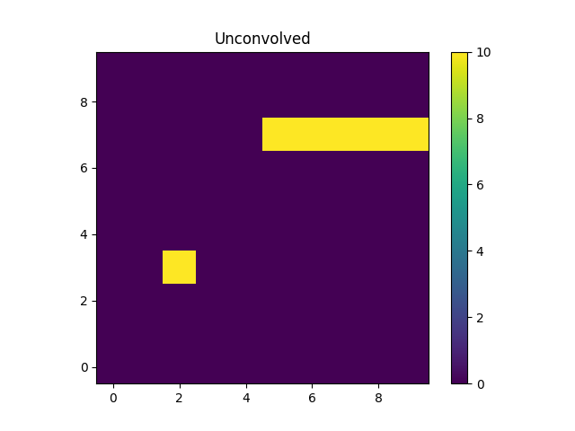
The “point source” is located at x = 2, y = 3 and the line
starts at x=5 and extends to the end of the grid (at y=7).
Note
In this example the image coordinates were chosen to be the same
as those drawn by matplotlib. The extent parameter of the
imshow call can be used when this correspondence does not
hold.
As with the 1D case, the
fold() method must be called
before evaluation.
>>> psf.fold(blank)
>>> m2 = blank.eval_model(convolved_mdl).reshape(xg.shape)
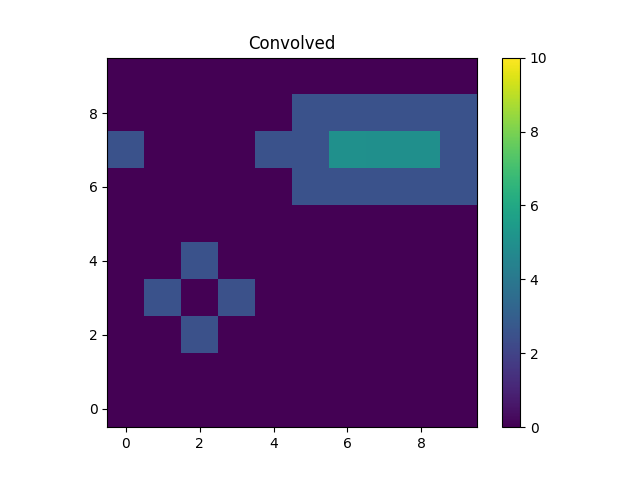
The kernel used redistributes flux from the central pixel to its four
immediate neighbors equally, which is what has happened to the point
source at (2, 2). The result for the line is to blur the line
slightly, but note that the convolution has “wrapped around”, so that
the flux that should have been placed into the pixel at (10, 7),
which is off the grid, has been moved to (0, 7).
Note
If the fold method is not called then evaluating the model will
raise the following exception:
PSFErr: PSF model has not been folded
Care must be taken to ensure that fold is called whenever the grid
has changed. This suggests that the same PSF model should not be used
in simultaneous fits, unless it is known that the grid is the same
in the multiple datasets.
The PSF Normalization
Since the norm parameter of the PSF model was set to 1, the PSF
convolution is flux preserving, even at the edges thanks to the
wrap-around behavior of the fourier transform. This can be seen by
comparing the signal in the unconvolved and convolved images, which
are (to numerical precision) the same:
>>> print(m1.sum())
58.0
>>> print(m2.sum())
58.0
The use of a fourier transform means that low-level signal will be
found in many pixels which would expect to be 0. For example,
looking at the row of pixels at y = 7 gives:
>>> m2[7]
array([2.50000000e+00, 1.73472348e-16, 5.20417043e-16, 4.33680869e-16,
       2.50000000e+00, 2.50000000e+00, 5.00000000e+00, 5.00000000e+00,
       5.00000000e+00, 2.50000000e+00])