Markov Chain Monte Carlo and Poisson data
Statistical background and Sherpa’s implementation
Sherpa provides a Markov Chain Monte Carlo (MCMC) method designed for Poisson-distributed data. It was originally developed as the Bayesian Low-Count X-ray Spectral (pyBLoCXS) [1] package based on the algorithm presented in Analysis of Energy Spectra with Low Photon Counts via Bayesian Posterior Simulation by van Dyk et al. (2001) [2]. A general description of the techniques employed along with their convergence diagnostics can be found in the Appendices of [2] and in [3].
Sherpa’s implementation of MCMC is written specifically for the Bayesian analysis. It supports a flexible definition of priors. It can be used to compute posterior predictive p-values for the likelihood ratio test [4]. It can also account for instrument calibration uncertainty [5].
MCMC selects random samples from the posterior probability
distribution for the assumed model starting from the best fit (maximum likelihood)
given by the standard optimization methods in Sherpa (i.e. result of the fit).
The MCMC is run using get_draws for a specific dataset, the selected sampler, the priors, and the specified number of iterations.
It returns an array of statistic values, an array of acceptance Booleans,
and an array of sampled parameter values (i.e. draws) from the posterior distribution.
The multivariate t-distribution is the default proposal distribution in get_draws.
This distribution is defined by the multivariate normal (for the model parameter values and the covariance matrix),
and chi2 distribution for a given degrees of freedom. The algorithm provides a choice of MCMC samplers with different
jumping rules for acceptance of the proposed parameters: Metropolis (symmetric) and Metropolis-Hastings (asymmetric).
Note that the multivariate normal distribution which requires the parameter values and
the corresponding covariance matrix. covar should be run beforehand.
Additional scale parameter allows to adjust the scale size of the multivariate normal in the definition of the t-distribution. This could improve the efficiency of the sampler and can be used to obtain the required acceptance rates.
Jumping Rules
The jumping rule determines how each step in the MCMC is calculated [3].
The setting can be changed using set_sampler. The sherpa.sim module provides
the following rules, which may be augmented by other modules:
MHuses a Metropolis-Hastings jumping rule assuming a multivariate t-distribution centered on the best-fit parameters.MetropolisMHmixes the Metropolis-Hastings jumping rule with the Metropolis jumping rule centered at the current set of parameters, in both cases sampled from the same t-distribution as used withMH. The probability of using the best-fit location as the start of the jump is given by thep_Mparameter of the rule (useget_samplerorget_sampler_optto view andset_sampler_optto set this value), otherwise the jump is from the previous location in the chain.
Options for the sampler are retrieved and set by get_sampler or
get_sampler_opt, and set_sampler_opt respectively. The list of
available samplers is given by list_samplers.
Choosing priors
By default, the prior on each parameter is taken to be flat, varying
from the parameter minima to maxima values. This prior can be changed
using the set_prior function, which can set the prior for a
parameter to a function or Sherpa model. The list of currently set
prior-parameter pairs is returned by the list_priors function, and the
prior function associated with a particular Sherpa model parameter may be
accessed with get_prior.
Running the chain
The get_draws function runs a chain using fit information
associated with the specified data set(s), and the currently set sampler and
parameter priors, for a specified number of iterations. It returns an array of
statistic values, an array of acceptance Booleans, and a 2-D array of
associated parameter values.
Analyzing the results
The sherpa.sim module contains several routines to visualize the results of the chain,
including plot_trace, plot_cdf, and plot_pdf, along with
get_error_estimates for calculating the limits from a
parameter chain.
References
Example
Simulate the data
Create a simulated data set:
>>> import numpy as np
>>> rng = np.random.RandomState(2)  # For reproducibility of this example
>>> x0low, x0high = 3000, 4000
>>> x1low, x1high = 4000, 4800
>>> dx = 15
>>> x1, x0 = np.mgrid[x1low:x1high:dx, x0low:x0high:dx]
Convert to 1D arrays:
>>> shape = x0.shape
>>> x0, x1 = x0.flatten(), x1.flatten()
Create the model used to simulate the data:
>>> from sherpa.astro.models import Beta2D
>>> truth = Beta2D()
>>> truth.xpos, truth.ypos = 3512, 4418
>>> truth.r0, truth.alpha = 120, 2.1
>>> truth.ampl = 12
Evaluate the model to calculate the expected values:
>>> mexp = truth(x0, x1).reshape(shape)
Create the simulated data by adding in Poisson-distributed noise:
>>> msim = rng.poisson(mexp)
What does the data look like?
Use an arcsinh transform to view the data, based on the work of Lupton, Gunn & Szalay (1999).
>>> import matplotlib.pyplot as plt
>>> # plt.image returns an image object. We don't need it any further for
>>> # this example, so we just put it in a throwaway variable to avoid extra screen output.
>>> _ = plt.imshow(np.arcsinh(msim), origin='lower', cmap='viridis',
...            extent=(x0low, x0high, x1low, x1high),
...            interpolation='nearest', aspect='auto')
>>> _ = plt.title('Simulated image')

Find the starting point for the MCMC
Set up a model and use the standard Sherpa approach to find a good starting place for the MCMC analysis:
>>> from sherpa import data, stats, optmethods, fit
>>> d = data.Data2D('sim', x0, x1, msim.flatten(), shape=shape)
>>> mdl = Beta2D()
>>> mdl.xpos, mdl.ypos = 3500, 4400
Use a Likelihood statistic and Nelder-Mead algorithm:
>>> f = fit.Fit(d, mdl, stats.Cash(), optmethods.NelderMead())
>>> res = f.fit()
>>> print(res.format())
Method                = neldermead
Statistic             = cash
Initial fit statistic = 20048.5
Final fit statistic   = 607.229 at function evaluation 777
Data points           = 3618
Degrees of freedom    = 3613
Change in statistic   = 19441.3
   beta2d.r0      121.945
   beta2d.xpos    3511.99
   beta2d.ypos    4419.72
   beta2d.ampl    12.0598
   beta2d.alpha   2.13319
Now calculate the covariance matrix (the default error estimate):
>>> f.estmethod
<Covariance error-estimation method instance 'covariance'>
>>> eres = f.est_errors()
>>> print(eres.format())
Confidence Method     = covariance
Fitting Method        = neldermead
Statistic             = cash
covariance 1-sigma (68.2689%) bounds:
   Param            Best-Fit  Lower Bound  Upper Bound
   -----            --------  -----------  -----------
   beta2d.r0         121.945     -7.12579      7.12579
   beta2d.xpos       3511.99     -2.09145      2.09145
   beta2d.ypos       4419.72     -2.10775      2.10775
   beta2d.ampl       12.0598    -0.610294     0.610294
   beta2d.alpha      2.13319    -0.101558     0.101558
The covariance matrix is stored in the extra_output attribute:
>>> cmatrix = eres.extra_output
>>> pnames = [p.split('.')[1] for p in eres.parnames]
>>> _ = plt.imshow(cmatrix, interpolation='nearest', cmap='viridis')
>>> _ = plt.xticks(np.arange(5), pnames)
>>> _ = plt.yticks(np.arange(5), pnames)
>>> _ = plt.colorbar()
Run the chain
Finally, run a chain (use a small number to keep the run time low for this example):
>>> from sherpa.sim import MCMC
>>> mcmc = MCMC()
>>> mcmc.get_sampler_name()
'MetropolisMH'
>>> draws = mcmc.get_draws(f, cmatrix, niter=1000, rng=rng)
>>> svals, accept, pvals = draws
>>> pvals.shape
(5, 1001)
Trace plots
>>> _ = plt.plot(pvals[0, :])
>>> _ = plt.xlabel('Iteration')
>>> _ = plt.ylabel('r0')

Or using the sherpa.plot module:
>>> from sherpa import plot
>>> tplot = plot.TracePlot()
>>> tplot.prepare(svals, name='Statistic')
>>> tplot.plot()

PDF of a parameter
>>> pdf = plot.PDFPlot()
>>> pdf.prepare(pvals[1, :], 20, False, 'xpos', name='example')
>>> pdf.plot()
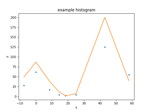
And adding in the covariance estimate using matplotlib.pyplot.annotate:
>>> xlo= eres.parmins[1] + eres.parvals[1]
>>> xhi = eres.parmaxes[1] + eres.parvals[1]
>>> _ = plt.annotate('', (xlo, 90), (xhi, 90), arrowprops={'arrowstyle': '<->'})
>>> _ = plt.plot([eres.parvals[1]], [90], 'ok')
CDF for a parameter
Normalise by the actual answer to make it easier to see how well the results match reality:
>>> cdf = plot.CDFPlot()
>>> _ = plt.subplot(2, 1, 1)
>>> cdf.prepare(pvals[1, :] - truth.xpos.val, r'$\Delta x$')
>>> cdf.plot(clearwindow=False)
>>> _ = plt.title('')
>>> _ = plt.subplot(2, 1, 2)
>>> cdf.prepare(pvals[2, :] - truth.ypos.val, r'$\Delta y$')
>>> cdf.plot(clearwindow=False)
>>> _ = plt.title('')
>>> plt.subplots_adjust(hspace=0.4)

Scatter plot
>>> _ = plt.scatter(pvals[0, :] - truth.r0.val,
...             pvals[4, :] - truth.alpha.val, alpha=0.3)
>>> _ = plt.xlabel(r'$\Delta r_0$', size=18)
>>> _ = plt.ylabel(r'$\Delta \alpha$', size=18)

This can be compared to the
RegionProjection calculation:
>>> _ = plt.scatter(pvals[0, :], pvals[4, :], alpha=0.3)
>>> from sherpa.plot import RegionProjection
>>> rproj = RegionProjection()
>>> rproj.prepare(min=[95, 1.8], max=[150, 2.6], nloop=[21, 21])
>>> rproj.calc(f, mdl.r0, mdl.alpha)
>>> rproj.contour(overplot=True)
>>> _ = plt.xlabel(r'$r_0$')
>>> _ = plt.ylabel(r'$\alpha$')

Connections to ArviZ
ArviZ is a Python package for exploratory analysis of Bayesian models.
It serves as a backend-agnostic tool for diagnosing and visualizing Bayesian inference and
provides different plotting and statistical diagnostic functions for MCMC chains that
are not implemented in Sherpa itself. If the ArviZ package is installed,
mcmc_to_arviz can be used to convert the MCMC results to a
DataTree object, which is the data structure that all
ArviZ routines use.
>>> import arviz as az
>>> from sherpa.sim import mcmc_to_arviz
>>> dataset = mcmc_to_arviz(mcmc=mcmc, fit=f, list_of_draws=[draws])
>>> _ = az.plot_pair(dataset)

See the ArviZ documentation for more details on the available plotting functions and statistical diagnostics.
Reference/API
- The sherpa.sim module
- The sherpa.sim.mh module
- The sherpa.sim.sample module
- NormalParameterSampleFromScaleMatrix
- NormalParameterSampleFromScaleVector
- NormalSampleFromScaleMatrix
- NormalSampleFromScaleVector
- ParameterSampleFromScaleMatrix
- ParameterSampleFromScaleVector
- ParameterScale
- ParameterScaleMatrix
- ParameterScaleVector
- StudentTParameterSampleFromScaleMatrix
- StudentTSampleFromScaleMatrix
- UniformParameterSampleFromScaleVector
- UniformSampleFromScaleVector
- multivariate_t
- multivariate_cauchy
- normal_sample
- uniform_sample
- t_sample
- Class Inheritance Diagram
- The sherpa.sim.simulate module