Simple Interpolation
Overview
Although Sherpa allows you to fit complex models to complex data sets with complex statistics and complex optimisers, it can also be used for simple situations, such as interpolating a function. In this example a one-dimensional set of data is given - i.e. \((x_i, y_i)\) - and a polynomial of order 2 is fit to the data. The model is then used to interpolate (and extrapolate) values. The walk through ends with changing the fit to a linear model (i.e. polynomial of order 1) and a comparison of the two model fits.
Setting up
The following sections will load in classes from Sherpa as needed, but it is assumed that the following modules have been loaded:
>>> import numpy as np
>>> import matplotlib.pyplot as plt
Loading the data
The data is the following:
x |
y |
|---|---|
1 |
1 |
1.5 |
1.5 |
2 |
1.75 |
4 |
3.25 |
8 |
6 |
17 |
16 |
which can be “loaded” into Sherpa using the
Data1D class:
>>> from sherpa.data import Data1D
>>> x = [1, 1.5, 2, 4, 8, 17]
>>> y = [1, 1.5, 1.75, 3.25, 6, 16]
>>> d = Data1D('interpolation', x, y)
>>> print(d)
name      = interpolation
x         = Float64[6]
y         = Float64[6]
staterror = None
syserror  = None
None
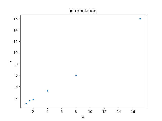
This can be displayed using the DataPlot class:
>>> from sherpa.plot import DataPlot
>>> dplot = DataPlot()
>>> dplot.prepare(d)
>>> dplot.plot()
Setting up the model
For this example, a second-order polynomial is going to be fit to the
data by using the Polynom1D class:
>>> from sherpa.models.basic import Polynom1D
>>> mdl = Polynom1D()
>>> print(mdl)
polynom1d
   Param        Type          Value          Min          Max      Units
   -----        ----          -----          ---          ---      -----
   polynom1d.c0 thawed            1 -3.40282e+38  3.40282e+38
   polynom1d.c1 frozen            0 -3.40282e+38  3.40282e+38
   polynom1d.c2 frozen            0 -3.40282e+38  3.40282e+38
   polynom1d.c3 frozen            0 -3.40282e+38  3.40282e+38
   polynom1d.c4 frozen            0 -3.40282e+38  3.40282e+38
   polynom1d.c5 frozen            0 -3.40282e+38  3.40282e+38
   polynom1d.c6 frozen            0 -3.40282e+38  3.40282e+38
   polynom1d.c7 frozen            0 -3.40282e+38  3.40282e+38
   polynom1d.c8 frozen            0 -3.40282e+38  3.40282e+38
   polynom1d.offset frozen            0 -3.40282e+38  3.40282e+38
The help for Polynom1D shows that the model is defined as:
so to get a second-order polynomial we have to
thaw the c2
parameter (the linear term c1 is kept at 0 to show that the
choice of parameter to fit is up to the user):
>>> mdl.c2.thaw()
This model can be compared to the data using the
ModelPlot class (note that, unlike
the data plot, the
prepare() method takes both
the data - needed to know what \(x_i\) to use - and the model):
>>> from sherpa.plot import ModelPlot
>>> mplot = ModelPlot()
>>> mplot.prepare(d, mdl)
>>> dplot.plot()
>>> mplot.overplot()
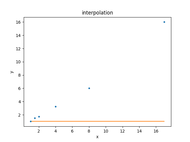
Since the default parameter values are still being used, the result is not a good description of the data. Let’s fix this!
Fitting the model to the data
Since we have no error bars, we are going to use least-squares
minimisation - that is, minimise the square of the distance between
the model and the data using the
LeastSq statisic and the
NelderMead optimiser
(for this case the LevMar optimiser is likely
to produce as good a result but faster, but I have chosen to
select the more robust method):
>>> from sherpa.stats import LeastSq
>>> from sherpa.optmethods import NelderMead
>>> from sherpa.fit import Fit
>>> f = Fit(d, mdl, stat=LeastSq(), method=NelderMead())
>>> print(f)
data      = interpolation
model     = polynom1d
stat      = LeastSq
method    = NelderMead
estmethod = Covariance
In this case there is no need to change any of the options for the
optimiser (the least-squares statistic has no options), so the objects
are passed straight to the Fit object.
The fit() method is used to fit the data; as it
returns useful information (in a FitResults
object) we capture this in the res variable, and then check that
the fit was successful (i.e. it converged):
>>> res = f.fit()
>>> res.succeeded
True
For this example the time to perform the fit is very short, but for complex data sets and models the call can take a long time!
A quick summary of the fit results is available via the
format() method, while printing the
variable retutrns more details:
>>> print(res.format())
Method                = neldermead
Statistic             = leastsq
Initial fit statistic = 255.875
Final fit statistic   = 2.4374 at function evaluation 264
Data points           = 6
Degrees of freedom    = 4
Change in statistic   = 253.438
   polynom1d.c0   1.77498
   polynom1d.c2   0.0500999
>>> print(res)
datasets       = None
itermethodname = none
methodname     = neldermead
statname       = leastsq
succeeded      = True
parnames       = ('polynom1d.c0', 'polynom1d.c2')
parvals        = (1.7749826216226083, 0.050099944904353017)
statval        = 2.4374045728256455
istatval       = 255.875
dstatval       = 253.43759542717436
numpoints      = 6
dof            = 4
qval           = None
rstat          = None
message        = Optimization terminated successfully
nfev           = 264
The best-fit parameter values can also be retrieved from the model itself:
>>> print(mdl)
polynom1d
   Param        Type          Value          Min          Max      Units
   -----        ----          -----          ---          ---      -----
   polynom1d.c0 thawed      1.77498 -3.40282e+38  3.40282e+38
   polynom1d.c1 frozen            0 -3.40282e+38  3.40282e+38
   polynom1d.c2 thawed    0.0500999 -3.40282e+38  3.40282e+38
   polynom1d.c3 frozen            0 -3.40282e+38  3.40282e+38
   polynom1d.c4 frozen            0 -3.40282e+38  3.40282e+38
   polynom1d.c5 frozen            0 -3.40282e+38  3.40282e+38
   polynom1d.c6 frozen            0 -3.40282e+38  3.40282e+38
   polynom1d.c7 frozen            0 -3.40282e+38  3.40282e+38
   polynom1d.c8 frozen            0 -3.40282e+38  3.40282e+38
   polynom1d.offset frozen            0 -3.40282e+38  3.40282e+38
as can the current fit statistic (as this is for fitting a second-order polynomial I’ve chosen to label the variable with a suffix of 2, which will make more sense below):
>>> stat2 = f.calc_stat()
>>> print("Statistic = {:.4f}".format(stat2))
Statistic = 2.4374
Note
In an actual analysis session the fit would probably be repeated, perhaps with a different optimiser, and starting from a different set of parameter values, to give more confidence that the fit has not been caught in a local minimum. This example is simple enough that this is not needed here.
To compare the new model to the data I am going to use a
FitPlot - which combines a DataPlot
and ModelPlot - and a ResidPlot - to look
at the residuals, defined as \({\rm data}_i - {\rm model}_i\),
using the SplitPlot class to orchestrate
the display (note that mplot needs to be re-created since the
model has changed since the last time its prepare method
was called):
>>> from sherpa.plot import FitPlot, ResidPlot, SplitPlot
>>> fplot = FitPlot()
>>> mplot.prepare(d, mdl)
>>> fplot.prepare(dplot, mplot)
>>> splot = SplitPlot()
>>> splot.addplot(fplot)
>>> rplot = ResidPlot()
>>> rplot.prepare(d, mdl, stat=LeastSq())
WARNING: The displayed errorbars have been supplied with the data or calculated using chi2xspecvar; the errors are not used in fits with leastsq
>>> rplot.plot_prefs['yerrorbars'] = False
>>> splot.addplot(rplot)
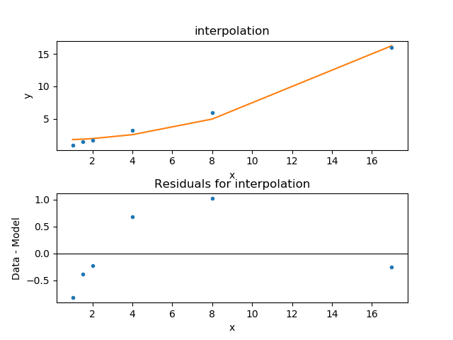
The default behavior for the residual plot is to include error bars,
here calculated using the Chi2XspecVar class,
but they have been turned off - by setting the
yerrorbars option to False - since they are not meaningful here.
Interpolating values
The model can be evaluated directly by supplying it with the independent-axis values; for instance for \(x\) equal to 2, 5, and 10:
>>> print(mdl([2, 5, 10]))
[1.9753824  3.02748124 6.78497711]
It can also be used to extrapolate the model outside the range of the data (as long as the model is defined for these values):
>>> print(mdl([-100]))
[502.77443167]
>>> print(mdl([234.56]))
[2758.19347071]
Changing the fit
Let’s see how the fit looks if we use a linear model instead. This
means thawing out the c1 parameter and clearing c2:
>>> mdl.c1.thaw()
>>> mdl.c2 = 0
>>> mdl.c2.freeze()
>>> f.fit()
<Fit results instance>
As this is a simple case, I am ignoring the return value from the
fit() method, but in an actual analysis
session it should be checked to ensure the fit converged.
The new model parameters are:
>>> print(mdl)
polynom1d
   Param        Type          Value          Min          Max      Units
   -----        ----          -----          ---          ---      -----
   polynom1d.c0 thawed    -0.248624 -3.40282e+38  3.40282e+38
   polynom1d.c1 thawed     0.925127 -3.40282e+38  3.40282e+38
   polynom1d.c2 frozen            0 -3.40282e+38  3.40282e+38
   polynom1d.c3 frozen            0 -3.40282e+38  3.40282e+38
   polynom1d.c4 frozen            0 -3.40282e+38  3.40282e+38
   polynom1d.c5 frozen            0 -3.40282e+38  3.40282e+38
   polynom1d.c6 frozen            0 -3.40282e+38  3.40282e+38
   polynom1d.c7 frozen            0 -3.40282e+38  3.40282e+38
   polynom1d.c8 frozen            0 -3.40282e+38  3.40282e+38
   polynom1d.offset frozen            0 -3.40282e+38  3.40282e+38
and the best-fit statistic value can be compared to the earlier version:
>>> stat1 = f.calc_stat()
>>> print("Statistic: order 1 = {:.3f} order 2 = {:.3f}".format(stat1, stat2))
Statistic: order 1 = 1.898 order 2 = 2.437
Note
Sherpa provides several routines for comparing statistic values,
such as sherpa.utils.calc_ftest() and
sherpa.utils.calc_mlr(), to see if one can be preferred
over the other, but these are not relevant here, as the statistic
being used is just the least-squared difference.
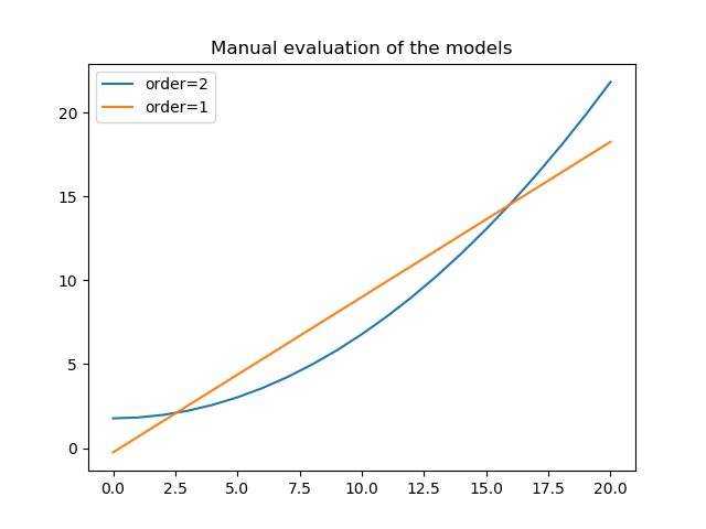
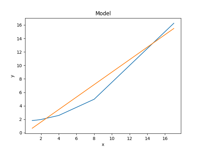
The two models can be visually compared by taking advantage of the previous plot objects retaining the values from the previous fit:
>>> mplot2 = ModelPlot()
>>> mplot2.prepare(d, mdl)
>>> mplot.plot()
>>> mplot2.overplot()
An alternative would be to create the plots directly (the
order=2 parameter values are restored from the res object
created from the first fit
to the data), in which case we are not limited to calculating the
model on the independent axis of the input data (the order is chosen
to match the colors of the previous plot):
>>> xgrid = np.linspace(0, 20, 21)
>>> y1 = mdl(xgrid)
>>> mdl.c0 = res.parvals[0]
>>> mdl.c1 = 0
>>> mdl.c2 = res.parvals[1]
>>> y2 = mdl(xgrid)
>>> plt.clf()
>>> plt.plot(xgrid, y2, label='order=2');
>>> plt.plot(xgrid, y1, label='order=1');
>>> plt.legend();
>>> plt.title("Manual evaluation of the models");