Simple user model
This example works through a fit to a small one-dimensional dataset which includes errors. This means that, unlike the Simple Interpolation example, an analysis of the parameter errors can be made. The fit begins with the use of the basic Sherpa models, but this turns out to be sub-optimal - since the model parameters do not match the required parameters - so a user model is created, which recasts the Sherpa model parameters into the desired form. It also has the advantage of simplifying the model, which avoids the need for manual intervention required with the Sherpa version.
Introduction
For this example, a data set from the literature was chosen, looking at non-Astronomy papers to show that Sherpa can be used in a variety of fields. There is no attempt made here to interpret the results, and the model parameters, and their errors, derived here should not be assumed to have any meaning compared to the results of the paper.
The data used in this example is taken from
Zhao Y, Tang X, Zhao X, Wang Y (2017) Effect of various nitrogen
conditions on population growth, temporary cysts and cellular biochemical
compositions of Karenia mikimotoi. PLoS ONE 12(2): e0171996.
doi:10.1371/journal.pone.0171996. The
Supporting information section of the paper includes a
spreadsheet containing the data for the figures, and this was
downloaded and stored as the file pone.0171996.s001.xlsx.
The aim is to fit a similar model to that described in Table 5, that is
where \(t\) and \(y\) are the abscissa (independent axis) and ordinate (dependent axis), respectively. The idea is to see if we can get a similar result rather than to make any inferences based on the data. For this example only the “NaNO3” dataset is going to be used.
Setting up
Both NumPy and Matplotlib are required:
>>> import numpy as np
>>> import matplotlib.pyplot as plt
Reading in the data
The openpyxl package (version 2.5.3) is used to read in the data from the Excel spreadsheet. This is not guaranteed to be the optimal means of reading in the data (and relies on hard-coded knowledge of the column numbers):
>>> from openpyxl import load_workbook
>>> wb = load_workbook('pone.0171996.s001.xlsx')
>>> fig4 = wb['Fig4data']
>>> t = []; y = []; dy = []
>>> for r in list(fig4.values)[2:]:
...     t.append(r[0])
...     y.append(r[3])
...     dy.append(r[4])
...
With these arrays, a data object can be created:
>>> from sherpa.data import Data1D
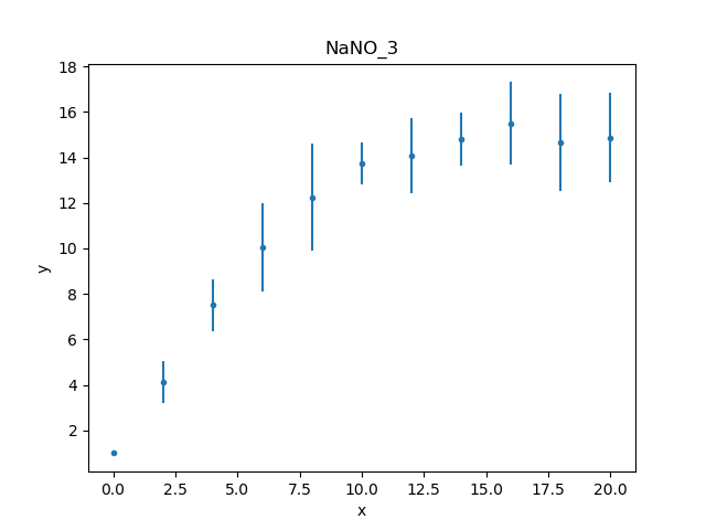
>>> d = Data1D('NaNO_3', t, y, dy)
Unlike the first worked example,
this data set includes an error column, so the data plot
created by DataPlot contains
error bars (although not obvious for the first point,
which has an error of 0):
>>> from sherpa.plot import DataPlot
>>> dplot = DataPlot()
>>> dplot.prepare(d)
>>> dplot.plot()
The data can also be inspected directly (as there aren’t many data points):
>>> print(d)
name      = NaNO_3
x         = Int64[11]
y         = Float64[11]
staterror = [0, 0.9214, 1.1273, 1.9441, 2.3363, 0.9289, 1.6615, 1.1726, 1.8066, 2.149, 1.983]
syserror  = None
Restricting the data
Trying to fit the whole data set will fail because the first data
point has an error of 0, so it is necessary to
restrict, or filter out,
this data point. The simplest way is to select a data range to ignore using
ignore(), in this
case everything where \(x < 1\):
>>> d.get_filter()
'0.0000:20.0000'
>>> d.ignore(None, 1)
>>> d.get_filter()
'2.0000:20.0000'
The get_filter() routine returns a
text description of the filters applied to the data; it starts
with all the data being included (0 to 20) and then after
excluding all points less than 1 the filter is now 2 to 20.
The format can be changed to something more appropriate for
this data set:
>>> d.get_filter(format='%d')
'2:20'
Since the data has been changed, the data plot object is updated so that the following plots reflect the new filter:
>>> dplot.prepare(d)
Creating the model
Table 5 lists the model fit to this dataset as
which can be constructed from components using the
Const1D
and Exp models, as shown below:
>>> from sherpa.models.basic import Const1D, Exp
>>> plateau = Const1D('plateau')
>>> rise = Exp('rise')
>>> mdl = plateau / (1 + rise)
>>> print(mdl)
(plateau / (1 + rise))
   Param        Type          Value          Min          Max      Units
   -----        ----          -----          ---          ---      -----
   plateau.c0   thawed            1 -3.40282e+38  3.40282e+38
   rise.offset  thawed            0 -3.40282e+38  3.40282e+38
   rise.coeff   thawed           -1 -3.40282e+38  3.40282e+38
   rise.ampl    thawed            1            0  3.40282e+38
The amplitude of the exponential is fixed at 1, but the other
terms will remain free in the fit, with plateau.c0 representing
the normalization, and the rise.offset and rise.coeff terms
the exponent term. The offset and coeff terms do not
match the form used in the paper, namely \(a + b t\),
which has some interesting consequences for the fit, as will
be discussed below in the
user-model section.
>>> rise.ampl.freeze()
>>> print(mdl)
(plateau / (1 + rise))
   Param        Type          Value          Min          Max      Units
   -----        ----          -----          ---          ---      -----
   plateau.c0   thawed            1 -3.40282e+38  3.40282e+38
   rise.offset  thawed            0 -3.40282e+38  3.40282e+38
   rise.coeff   thawed           -1 -3.40282e+38  3.40282e+38
   rise.ampl    frozen            1            0  3.40282e+38
The functional form of the exponential model provided by Sherpa, assuming an amplitude of unity, is
which means that I expect the final values to be \({\rm coeff} \simeq -0.5\) and, as \(- {\rm coeff} * {\rm offset} \simeq 1.9\), then \({\rm offset} \simeq 4\). The plateau value should be close to 15.
The model and data can be shown together, but as the fit has not yet been made then showing on the same plot is not very instructive, so here’s two plots one above the other, created by mixing the Sherpa and Matplotlib APIs:
>>> from sherpa.plot import ModelPlot
>>> mplot = ModelPlot()
>>> mplot.prepare(d, mdl)
>>> plt.subplot(2, 1, 1)
>>> mplot.plot(clearwindow=False)
>>> plt.subplot(2, 1, 2)
>>> dplot.plot(clearwindow=False)
>>> plt.title('')
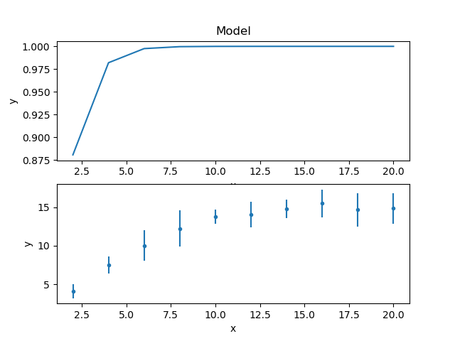
The title of the data plot was removed since it overlapped the X axis of the model plot above it.
Fitting the data
The main difference to fitting the first example is that the
Chi2 statistic is used,
since the data contains error values.
>>> from sherpa.stats import Chi2
>>> from sherpa.fit import Fit
>>> f = Fit(d, mdl, stat=Chi2())
>>> print(f)
data      = NaNO_3
model     = (plateau / (1 + rise))
stat      = Chi2
method    = LevMar
estmethod = Covariance
>>> print("Starting statistic: {}".format(f.calc_stat()))
Starting statistic: 633.2233812020354
The use of a Chi-square statistic means that the fit also calculates the reduced statistic (the final statistic value divided by the degrees of freedom), which should be \(\sim 1\) for a “good” fit, and an estimate of the probability (Q value) that the fit is good (this is also based on the statistic and number of degrees of freedom).
>>> fitres = f.fit()
>>> print(fitres.format())
Method                = levmar
Statistic             = chi2
Initial fit statistic = 633.223
Final fit statistic   = 101.362 at function evaluation 17
Data points           = 10
Degrees of freedom    = 7
Probability [Q-value] = 5.64518e-19
Reduced statistic     = 14.4802
Change in statistic   = 531.862
   plateau.c0     10.8792      +/- 0.428815
   rise.offset    457.221      +/- 0
   rise.coeff     24.3662      +/- 0
Changed in version 4.10.1: The implementation of the LevMar
class has been changed from Fortran to C++ in the 4.10.1 release.
The results of the optimiser are expected not to change
significantly, but one of the more-noticeable changes is that
the covariance matrix is now returned directly from a fit,
which results in an error estimate provided as part of the
fit output (the values after the +/- terms above).
The reduced chi-square value is large, as shown in the screen output above and the explicit access below, the probability value is essentially 0, and the parameters are nowhere near the expected values.
>>> print("Reduced chi square = {:.2f}".format(fitres.rstat))
Reduced chi square = 14.48
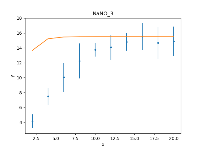
Visually comparing the model and data values highlights how poor
this fit is (the data plot does not need regenerating in this
case, but prepare() is called
just to make sure that the correct data is being displayed):
>>> dplot.prepare(d)
>>> mplot.prepare(d, mdl)
>>> dplot.plot()
>>> mplot.overplot()
Either the model has got caught in a local minimum, or it is not
a good description of the data. To investigate further, a useful technique
is to switch the optimiser and re-fit; the hope is that the different
optimiser will be able to escape the local minima in the search
space. The default optimiser used by
Fit is
LevMar, which is often a good
choice for data with errors. The other standard optimiser
provided by Sherpa is
NelderMead, which is often slower
than LevMar - as it requires more model evaluations - but
less-likely to get stuck:
>>> from sherpa.optmethods import NelderMead
>>> f.method = NelderMead()
>>> fitres2 = f.fit()
>>> print(mdl)
(plateau / (1 + rise))
   Param        Type          Value          Min          Max      Units
   -----        ----          -----          ---          ---      -----
   plateau.c0   thawed      10.8792 -3.40282e+38  3.40282e+38
   rise.offset  thawed      457.221 -3.40282e+38  3.40282e+38
   rise.coeff   thawed      24.3662 -3.40282e+38  3.40282e+38
   rise.ampl    frozen            1            0  3.40282e+38
An alternative to replacing the
method attribute, as done above, would be
to create a new Fit object - changing the
method using the method attribute of the initializer, and use
that to fit the model and data.
As can be seen, the parameter values have not changed; the
dstatval attribute contains the
change in the statsitic value, and as shown below, it has
not improved:
>>> fitres2.dstatval
0.0
The failure of this fit is actually down to the coupling of
the offset and coeff parameters of the
Exp model, as will be
discussed below,
but a good solution can be found by tweaking the starting
parameter values.
Restarting the fit
The reset() will change the
parameter values back to the
last values you set them to,
which may not be the same as their
default settings
(in this case the difference is in the state of the rise.ampl
parameter, which has remained frozen):
>>> mdl.reset()
>>> print(mdl)
(plateau / (1 + rise))
   Param        Type          Value          Min          Max      Units
   -----        ----          -----          ---          ---      -----
   plateau.c0   thawed            1 -3.40282e+38  3.40282e+38
   rise.offset  thawed            0 -3.40282e+38  3.40282e+38
   rise.coeff   thawed           -1 -3.40282e+38  3.40282e+38
   rise.ampl    frozen            1            0  3.40282e+38
Note
It is not always necessary to reset the parameter values when trying to get out of a local minimum, but it can be a useful strategy to avoid getting trapped in the same area.
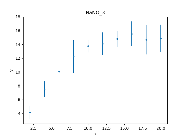
One of the simplest changes to make here is to set the plateau term to the maximum data value, as the intention is for this term to represent the asymptote of the curve.
>>> plateau.c0 = np.max(d.y)
>>> mplot.prepare(d, mdl)
>>> dplot.plot()
>>> mplot.overplot()
A new fit object could be created, but it is also possible
to reuse the existing object. This leaves the optimiser set to
NelderMead, although in this
case the same parameter values are found if the method
attribute had been changed back to
LevMar:
>>> fitres3 = f.fit()
>>> print(fitres3.format())
Method                = neldermead
Statistic             = chi2
Initial fit statistic = 168.42
Final fit statistic   = 0.299738 at function evaluation 42
Data points           = 10
Degrees of freedom    = 7
Probability [Q-value] = 0.9999
Reduced statistic     = 0.0428198
Change in statistic   = 168.12
   plateau.c0     14.9694      +/- 0.859633
   rise.offset    4.17729      +/- 0.630148
   rise.coeff     -0.420696    +/- 0.118487
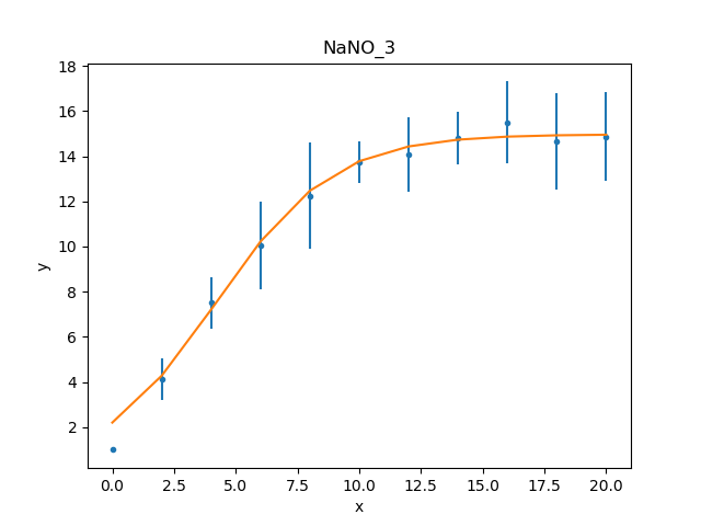
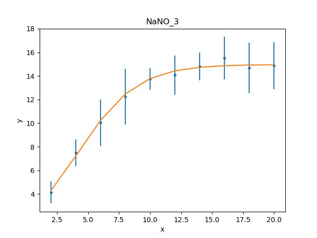
These results already look a lot better than the previous attempt; the reduced statistic is much smaller, and the values are similar to the reported values. As shown in the plot below, the model also well describes the data:
>>> mplot.prepare(d, mdl)
>>> dplot.plot()
>>> mplot.overplot()

The residuals can also be displayed, in this case normalizing by
the error values by using a
DelchiPlot plot:
>>> from sherpa.plot import DelchiPlot
>>> residplot = DelchiPlot()
>>> residplot.prepare(d, mdl, f.stat)
>>> residplot.plot()
Unlike the data and model plots, the
prepare() method of the
residual plot requires a statistic object, so the value
in the fit object (using the stat
attribute) is used.
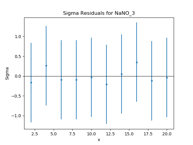
Given that the reduced statistic for the fit is a lot smaller than 1 (\(\sim 0.04\)), the residuals are all close to 0: the ordinate axis shows \((d - m) / e\) where \(d\), \(m\), and \(e\) are data, model, and error value respectively.
What happens at \(t = 0\)?
The filtering applied earlier
can be removed, to see how the model behaves at low times. Calling
the notice() without any arguments
removes any previous filter:
>>> d.notice()
>>> d.get_filter(format='%d')
'0:20'
For this plot, the FitPlot class is going
to be used to show both the data and model rather than doing it
manually as above:
>>> from sherpa.plot import FitPlot
>>> fitplot = FitPlot()
>>> dplot.prepare(d)
>>> mplot.prepare(d, mdl)
>>> fitplot.prepare(dplot, mplot)
>>> fitplot.plot()
Note
The prepare method on the
components of the Fit plot (in this case dplot and
mplot) must be called with their appropriate arguments
to ensure that the latest changes - such as filters and
parameter values - are picked up.
Warning
Trying to create a residual plot for this new data range,
will end up with a division-by-zero warning from the
prepare call, as the first data point has an error
of 0 and the residual plot shows \((d - m) / e\).
For the rest of this example the first data point has been removed:
>>> d.ignore(None, 1)
Estimating parameter errors
The calc_stat_info() method returns
an overview of the current fit:
>>> statinfo = f.calc_stat_info()
>>> print(statinfo)
name      =
ids       = None
bkg_ids   = None
statname  = chi2
statval   = 0.2997382864907501
numpoints = 10
dof       = 7
qval      = 0.999900257642653
rstat     = 0.04281975521296431
It is another way of getting at some of the information in the
FitResults object; for instance
>>> statinfo.rstat == fitres3.rstat
True
Note
The FitResults object refers to the model at the time
the fit was made, whereas calc_stat_info is calculated
based on the current values, and so the results can be
different.
The est_errors() method is used to
estimate error ranges for the parameter values. It does this by
varying the parameters around the best-fit location
until the statistic value has increased by a set amount.
The default method for estimating errors is
Covariance
>>> f.estmethod.name
'covariance'
which has the benefit of being fast, but may not be as robust as other techniques.
>>> coverrs = f.est_errors()
>>> print(coverrs.format())
Confidence Method     = covariance
Iterative Fit Method  = None
Fitting Method        = levmar
Statistic             = chi2
covariance 1-sigma (68.2689%) bounds:
   Param            Best-Fit  Lower Bound  Upper Bound
   -----            --------  -----------  -----------
   plateau.c0        14.9694    -0.880442     0.880442
   rise.offset       4.17729    -0.646012     0.646012
   rise.coeff      -0.420696     -0.12247      0.12247
These errors are similar to those reported during the fit.
As shown below,
the error values can be extracted from the output of
est_errors().
The default is to calculate “one sigma” error bounds
(i.e. those that cover 68.3% of the expected parameter range),
but this can be changed by altering the
sigma attribute
of the error estimator.
>>> f.estmethod.sigma
1
Changing this value to 1.6 means that the errors are close to the 90% bounds (for a single parameter):
>>> f.estmethod.sigma = 1.6
>>> coverrs90 = f.est_errors()
>>> print(coverrs90.format())
Confidence Method     = covariance
Iterative Fit Method  = None
Fitting Method        = neldermead
Statistic             = chi2
covariance 1.6-sigma (89.0401%) bounds:
   Param            Best-Fit  Lower Bound  Upper Bound
   -----            --------  -----------  -----------
   plateau.c0        14.9694     -1.42193      1.42193
   rise.offset       4.17729     -1.04216      1.04216
   rise.coeff      -0.420696     -0.19679      0.19679
The covariance method uses the covariance matrix to estimate
the error surface, and so the parameter errors are symmetric.
A more-robust, but often significantly-slower, approach is to
use the Confidence approach:
>>> from sherpa.estmethods import Confidence
>>> f.estmethod = Confidence()
>>> conferrs = f.est_errors()
plateau.c0 lower bound: -0.804259
rise.offset lower bound:     -0.590258
rise.coeff lower bound: -0.148887
rise.offset upper bound:     0.714407
plateau.c0 upper bound: 0.989664
rise.coeff upper bound: 0.103391
The error estimation for the confidence technique is run in parallel - if the machine has multiple cores usable by the Python multiprocessing module - which can mean that the screen output above is not always in the same order. As shown below, the confidence-derived error bounds are similar to the covariance bounds, but are not symmetric.
>>> print(conferrs.format())
Confidence Method     = confidence
Iterative Fit Method  = None
Fitting Method        = neldermead
Statistic             = chi2
confidence 1-sigma (68.2689%) bounds:
   Param            Best-Fit  Lower Bound  Upper Bound
   -----            --------  -----------  -----------
   plateau.c0        14.9694    -0.804259     0.989664
   rise.offset       4.17729    -0.590258     0.714407
   rise.coeff      -0.420696    -0.148887     0.103391
The default is to use all
thawed parameters
in the error analysis, but the est_errors()
method has a parlist attribute which can be used to restrict
the parameters used, for example to just the offset term:
>>> offseterrs = f.est_errors(parlist=(mdl.pars[1], ))
rise.offset lower bound:     -0.590258
rise.offset upper bound:     0.714407
>>> print(offseterrs)
datasets    = None
methodname  = confidence
iterfitname = none
fitname     = neldermead
statname    = chi2
sigma       = 1
percent     = 68.26894921370858
parnames    = ('rise.offset',)
parvals     = (4.177287700807689,)
parmins     = (-0.5902580352584237,)
parmaxes    = (0.7144070082643514,)
nfits       = 8
The covariance and confidence limits can be compared by
accessing the fields of the
ErrorEstResults object:
>>> fmt = "{:13s} covar=±{:4.2f}  conf={:+5.2f} {:+5.2f}"
>>> for i in range(len(conferrs.parnames)):
...     print(fmt.format(conferrs.parnames[i], coverrs.parmaxes[i],
...                      conferrs.parmins[i], conferrs.parmaxes[i]))
...
plateau.c0    covar=±0.88  conf=-0.80 +0.99
rise.offset   covar=±0.65  conf=-0.59 +0.71
rise.coeff    covar=±0.12  conf=-0.15 +0.10
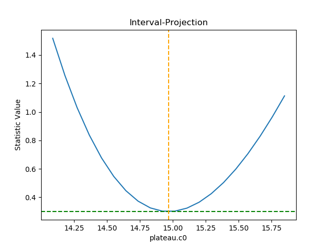
The est_errors() method returns a
range, but often it is important to visualize the error
surface, which can be done using the interval projection
(for one parameter) and region projection (for two parameter)
routines. The one-dimensional version is created with the
IntervalProjection
class, as shown in the following, which shows how the statistic
varies with the plateau term (the vertical dashed line indicates
the best-fit location for the parameter, and the horizontal
line the statistic value for the best-fit location):
>>> from sherpa.plot import IntervalProjection
>>> intproj = IntervalProjection()
>>> intproj.calc(f, plateau.c0)
>>> intproj.plot()
Unlike the previous plots, this requires calling the
calc() method
before plot(). As
the prepare()
method was not called, it used the default options to
calculate the plot range (i.e. the range over which
plateau.c0 would be varied), which turns out in this
case to be close to the one-sigma limits.
The range, and number of points, can also be set explicitly:
>>> intproj.prepare(min=12.5, max=20, nloop=51)
>>> intproj.calc(f, plateau.c0)
>>> intproj.plot()
>>> s0 = f.calc_stat()
>>> for ds in [1, 4, 9]:
...     intproj.hline(s0 + ds, overplot=True, linestyle='dot', linecolor='gray')
...
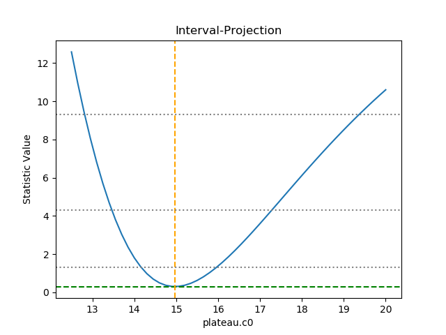
The horizontal lines indicate the statistic value for one, two, and three sigma limits for a single parameter value (and assuming a Chi-square statistic). The plot shows how, as the parameter moves away from its best-fit location, the search space becomes less symmetric.
Following the same approach, the RegionProjection
class calculates the statistic value as two parameters are varied,
displaying the results as a contour plot. It requires two parameters
and the visualization is
created with the contour()
method:
>>> from sherpa.plot import RegionProjection
>>> regproj = RegionProjection()
>>> regproj.calc(f, rise.offset, rise.coeff)
>>> regproj.contour()
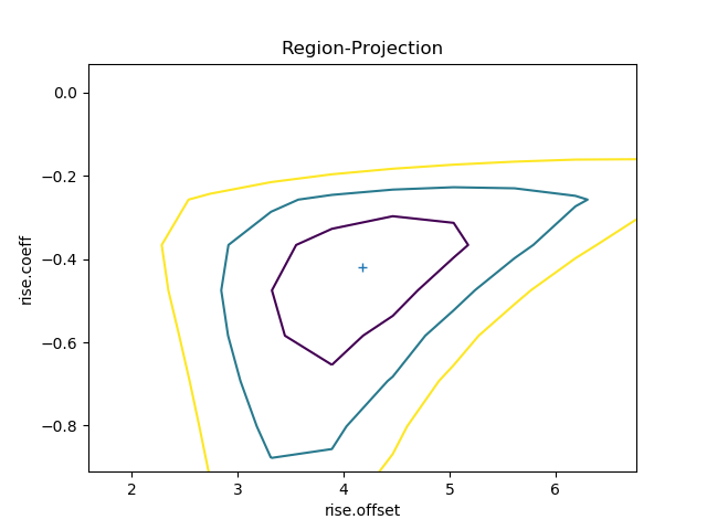
The contours show the one, two, and three sigma contours, with the
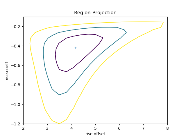
cross indicating the best-fit value. As with the interval-projection plot,
the prepare() method can
be used to define the grid of points to use; the values below are
chosen to try and cover the full three-sigma range as well as improve
the smoothness of the contours by increasing the number of points
that are looped over:
>>> regproj.prepare(min=(2, -1.2), max=(8, -0.1), nloop=(21, 21))
>>> regproj.calc(f, rise.offset, rise.coeff)
>>> regproj.contour()
Writing your own model
The approach above has provided fit results, but they do not match those of the paper and, since
it is hard to transform the values from above to get
accurate results. An alternative approach is to
create a model with the parameters
in the required form, which requires a small amount
of code (by using the
Exp class to do the actual
model evaluation).
The following class (MyExp) creates a model that has
two parameters (a and b) that represents
\(f(x) = e^{a + b x}\). The starting values for these
parameters are chosen to match the default values of the
Exp parameters,
where \({\rm coeff} = -1\) and \({\rm offset} = 0\):
from sherpa.models.basic import RegriddableModel1D
from sherpa.models.parameter import Parameter

class MyExp(RegriddableModel1D):
    """A simpler form of the Exp model.

    The model is f(x) = exp(a + b * x).
    """

    def __init__(self, name='myexp'):

        self.a = Parameter(name, 'a', 0)
        self.b = Parameter(name, 'b', -1)

        # The _exp instance is used to perform the model calculation,
        # as shown in the calc method.
        self._exp = Exp('hidden')

        return RegriddableModel1D.__init__(self, name, (self.a, self.b))

    def calc(self, pars, *args, **kwargs):
        """Calculate the model"""

        # Tell the exp model to evaluate the model, after converting
        # the parameter values to the required form, and order, of:
        # offset, coeff, ampl.
        #
        coeff = pars[1]
        offset = -1 * pars[0] / coeff
        ampl = 1.0
        return self._exp.calc([offset, coeff, ampl], *args, **kwargs)
This can be used as any other Sherpa model:
>>> plateau2 = Const1D('plateau2')
>>> rise2 = MyExp('rise2')
>>> mdl2 = plateau2 / (1 + rise2)
>>> print(mdl2)
(plateau2 / (1 + rise2))
   Param        Type          Value          Min          Max      Units
   -----        ----          -----          ---          ---      -----
   plateau2.c0  thawed            1 -3.40282e+38  3.40282e+38
   rise2.a      thawed            0 -3.40282e+38  3.40282e+38
   rise2.b      thawed           -1 -3.40282e+38  3.40282e+38
>>> fit2 = Fit(d, mdl2, stat=Chi2())
>>> res2 = fit2.fit()
>>> print(res2.format())
Method                = levmar
Statistic             = chi2
Initial fit statistic = 633.223
Final fit statistic   = 0.299738 at function evaluation 52
Data points           = 10
Degrees of freedom    = 7
Probability [Q-value] = 0.9999
Reduced statistic     = 0.0428198
Change in statistic   = 632.924
   plateau2.c0    14.9694      +/- 0.859768
   rise2.a        1.75734      +/- 0.419169
   rise2.b        -0.420685    +/- 0.118473

>>> dplot.prepare(d)
>>> mplot2 = ModelPlot()
>>> mplot2.prepare(d, mdl2)
>>> dplot.plot()
>>> mplot2.overplot()
Unlike the initial attempt,
this version did not require any manual intervention to find the
best-fit solution. This is because the degeneracy between the two
terms of the exponential in the
Exp model have been broken in
this version, and so the optimiser work better.
It also has the advantage that the parameters match the
problem, and so the parameter limits determined below can be
used directly, without having to transform them.
>>> fit2.estmethod = Confidence()
>>> conferrs2 = fit2.est_errors()
plateau2.c0 lower bound:     -0.804444
rise2.b lower bound: -0.148899
rise2.a lower bound: -0.38086
rise2.b upper bound: 0.10338
plateau2.c0 upper bound:     0.989623
rise2.a upper bound: 0.489919
>>> print(conferrs2.format())
Confidence Method     = confidence
Iterative Fit Method  = None
Fitting Method        = levmar
Statistic             = chi2
confidence 1-sigma (68.2689%) bounds:
   Param            Best-Fit  Lower Bound  Upper Bound
   -----            --------  -----------  -----------
   plateau2.c0       14.9694    -0.804444     0.989623
   rise2.a           1.75734     -0.38086     0.489919
   rise2.b         -0.420685    -0.148899      0.10338
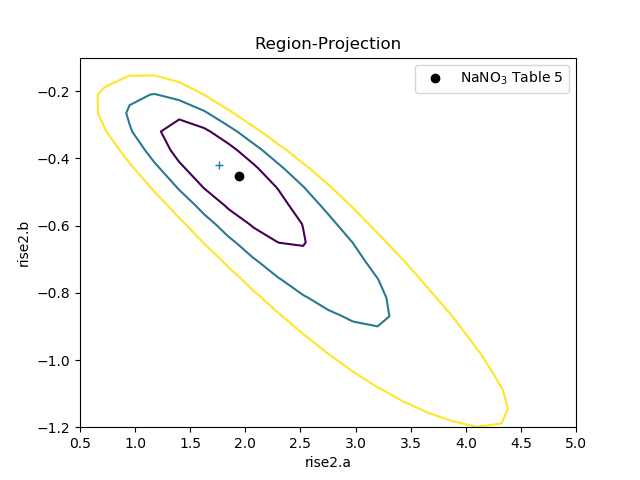
The difference in the model parameterisation can also be seen in the various error-analysis plots, such as the region-projection contour plot (where the limits have been chosen to cover the three-sigma contour), and a marker has been added to show the result listed in Table 5 of Zhao et al:
>>> regproj2 = RegionProjection()
>>> regproj2.prepare(min=(0.5, -1.2), max=(5, -0.1), nloop=(21, 21))
>>> regproj2.calc(fit2, rise2.a, rise2.b)
>>> regproj2.contour()
>>> plt.plot(1.941, -0.453, 'ko', label='NaNO$_3$ Table 5')
>>> plt.legend(loc=1)