Optimizing functions
The sherpa.optmethods module provides classes that let you
optimize models when applied to data instances, and this is handled by the fit module. You can apply the optimizers directly to
functions if you do not need to take advantage of Sherpa’s model and
data classes.
The optimizers in sherpa.optmethods.optfcts are functions
which follow the same interface:
optimizer(cb, start, lolims, hilims, **kwargs)
where cb is a callable that given a set or parameters returns the
current statistic, start is the starting positions of the
parameters, lolims and hilims are the bounds of the parameters,
and the remaining keyword arguments are specific to the optimizer.
These optimizers can be compared to SciPy’s optimiaztion routines.
Examples
The following imports have been made:
>>> import numpy as np
>>> from matplotlib import pyplot as plt
>>> from matplotlib import colors
>>> from mpl_toolkits.mplot3d import Axes3D
>>> from astropy.table import Table
>>> from sherpa.optmethods import optfcts
A simple function
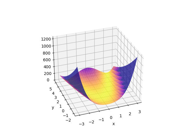
The function we want to optimize is a version of the
Rosenbrock function,
where a=2 and b=10, so the best-fit location is at:
x = a = 2
y = a**2 = 4
Note
The Sherpa test suite contains a number of test cases based on functions like this, taken from More, J. J., Garbow, B. S., and Hillstrom, K. E.. Testing unconstrained optimization software. United States: N. p., 1978. Web. doi:10.2172/6650344..
The SciPy optimization tutorial
uses a=1 and b=100.
The function is:
def rosenbrock(x, y):
    a, b = 2, 10
    return (a - x)**2 + b * (y - x**2)**2
We can look at the surface close to the best-fit location What does the function look like?
>>> y, x = np.mgrid[-2:5.1:0.1, -3:3.1:0.1]
>>> surface = rosenbrock(x, y)
>>> print(surface.shape)
(71, 61)
>>> print(surface.min())
0.0
>>> print(surface.max())
1235.0
This can be visualized as:
>>> fig, ax = plt.subplots(subplot_kw={"projection": "3d"})
>>> surf = ax.plot_surface(x, y, surface,
...                        cmap=cm.plasma_r, alpha=0.8,
...                        vlim=0, vmax=300)
>>> ax.set_xlabel('x')
>>> ax.set_ylabel('y')
>>> ax.view_init(30, -100)
In order to optimize this function we need to determine how we want to define the “search surface”; that is the value that the optimizer is going to try and minimize. For this dataset, where the minimum is 0, we can use the square of the function (i.e. a least-squares model). Now, the function we pass to the minimizer requires two values - the “statistic” and a per-parameter breakdown of the parameter - but for now we are going to ignore the latter, as it’s only needed for some optimizers. This gives us:
def to_optimize1(args):
    x = args[0]
    y = args[1]
    pa = (2 - x)**2
    pb = 10 * (y - x**2)**2
    stat = pa**2 + pb**2
    return stat, None
The function can then be minimized by passing the routine, the
starting point, and the bounds, to the optimizer - in this case the
minim routine:
>>> start = [-1.2, 1]
>>> lo = [-100, -100]
>>> hi = [100, 100]
>>> res = optfcts.minim(to_optimize1, start, lo, hi)
The return value is a tuple which contains a success flag, the best-fit parameters, the value at this location, a message, and a dictionary with optimizer-specific information:
>>> print(f"Success: {res[0]}")
Success: True
>>> print(f"Message: {res[3]}")
Message: successful termination
>>> print(f"extra:   {res[4]}")
extra:   {'info': 0, 'nfev': 80}
>>> print(f"best-fit location: {res[1]}")
best-fit location: [2.00219515 4.00935405]
>>> print(f"          minimum: {res[2]}")
          minimum: 3.3675019403007895e-11
So, the correct location is (2, 4) and we can see we got close.
As the different optimizers use the same interface we can easily try different optimizers:
>>> tbl = Table(names=['method', 'stat0', 'x', 'y'],
...             dtype=[str, float, float, float])
>>> for method in [optfcts.minim, optfcts.neldermead, optfcts.lmdif, optfcts.montecarlo]:
...     res = method(to_optimize1, start, lo, hi)
...     if res[0]:
...         tbl.add_row([method.__name__, res[2], res[1][0], res[1][1]])
...     else:
...         print(f"Failed {method.__name__}: {res[3]}")
...
Failed lmdif: improper input parameters
>>> print(tbl)
    method           stat0                 x                  y
  ---------- --------------------- ------------------ ------------------
     minim 3.3675019403007895e-11 2.0021951482261993 4.009354048420242
neldermead  1.269579878170357e-16  2.000079242383145  4.00028638884874
montecarlo  5.028337191787579e-16  2.000144877499188 4.000607622717231
In this particular case lmdif
failed, and this is because the to_optimize1 function returned None
as its second argument. For the other cases we can see that they all
found the minimum location.
In order to use lmdif we need
the per-parameter statistic, which we can get with a small tweak:
def to_optimize2(args):
    x = args[0]
    y = args[1]
    pa = (a - x)**2
    pb = b * (y - x**2)**2
    stat = pa**2 + pb**2
    return stat, [pa, pb]
This lets us use lmdif:
>>> res2 = optfcts.lmdif(to_optimize2, start, lo, hi)
>>> res2[0]
True
>>> res2[1]
[1.99240555 3.9690085 ]
The lmdif optimizer is one of those that returns a number of
elements in the “extra” dictionary:
>>> res2[4]
{'info': 0, 'nfev': 514, 'covar': array([[4.75572913e+03, 1.44740585e+06],
       [1.44740585e+06, 4.43876953e+08]]), 'num_parallel_map': 0}
Optimizing a model
We can re-create the Fitting the NormGauss1D and Lorentz1D models
section - at least for the NormGauss1D fit.
The normalized gaussian model can be expressed as
def ngauss(x, ampl, pos, fwhm):
    term = 4 * np.log(2)
    numerator = ampl * np.exp(-term * (x - pos)**2 / fwhm**2)
    denominator = np.sqrt(np.pi / term) * fwhm
    return numerator / denominator
and the data we are going to fit is read from a file:
>>> d = np.loadtxt('test_peak.dat')
>>> x = d[:, 0]
>>> y = d[:, 1]
In this case we want to minimize the least-squares difference between
the model - evaluated on the x axis - and the y values.
def cb(pars):
    model = ngauss(x, pars[0], pars[1], pars[2])
    delta = model - y
    statval = (delta * delta).sum()
    # Keep a record of the parameters we've visited
    store.add_row([statval] + list(pars))
    return statval, delta
Note
The use of store is not required here; it just lets the user
find out how the parameter space was searched, which will
be discussed below.
Users of the full Sherpa system to model and fit data can
take advantage of the outfile argument of the
sherpa.fit.Fit.fit method to save the per-iteration parameter
values.
This function would normally be written as a class or a closure to
ensure that the use of global terms like x, y, ngauss, and
store do not cause problems.
For the starting point and bounds let us use an estimate - in Sherpa
parameter terms a guess - based on the data:
>>> start = [y.max(), (x[0] + x[-1]) / 2, (x[-1] - x[0]) / 10]
>>> lows = [0, x[0], 0]
>>> his = [1e4, x[-1], x[-1] - x[0]]
which can be used with the neldermead optimizer:
>>> store = Table(names=['stat', 'ampl', 'pos', 'fwhm'])
>>> flag, bestfit, statval, msg, opts = optfcts.neldermead(cb, start, lows, his)
>>> flag
True
>>> print(bestfits)
[30.31354039  9.24277042  2.90156672]
>>> statval
29.994315740189727
>>> opts
{'info': True, 'nfev': 267}
>>> len(store)
267
and displayed:
>>> plt.plot(x, y, label='Data', alpha=0.5)
>>> plt.plot(x, ngauss(x, *start), label='Start')
>>> plt.plot(x, ngauss(x, *bestfit), label='Best fit', c='k')
>>> plt.legend()
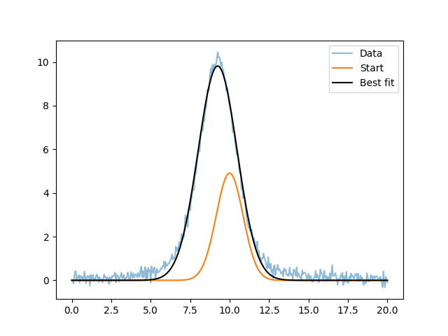
This result matches the Fitting the NormGauss1D and Lorentz1D models result. Note that at this point you are close to replicating the main parts of Sherpa (but with a lot-less functionality)!
One tweak that was added to the cb routine, compared to
to_optimize1 and to_optimize2, is the ability to store the
parameter values at each iteration:
>>> print(store)
       stat               ampl               pos                fwhm
------------------ ------------------ ----------------- -------------------
1995.1782885013076          10.452393              10.0                 2.0
1830.6327671752738          11.652393              10.0                 2.0
3522.2622560146397          10.452393              11.2                 2.0
  2156.39741128647          10.452393              10.0                 3.2
 1764.261448064872 11.252393000000001               8.8                 2.8
 2715.012206450446 11.652393000000004 7.600000000000001  3.1999999999999993
 1366.678033289349 11.785726333333333               9.2   1.333333333333333
  4770.95772056462          12.452393 8.799999999999997 0.39999999999999947
1504.4139142274962 12.674615222222219 8.666666666666668  2.0888888888888886
2731.7112487850172 12.156096703703703 7.777777777777779   2.148148148148148
1379.1243615097005 11.778318925925927 9.444444444444445   2.037037037037037
1946.1190085808503 12.906713987654314 9.407407407407408  0.8395061728395059
 1495.009488013458  11.66597324691358 8.951851851851853  2.3098765432098762
1684.8390859851572  10.81206378189301 9.730864197530863  1.6979423868312757
1355.3671486446174 12.208977362139915 8.932716049382716  1.9911522633744854
1399.8451502742626 12.182708500685873 9.432921810699586   1.264471879286694
1279.2923719811783 12.053524687242799 9.312654320987653  1.5258230452674897
1610.2269471113636 12.253833329218104 8.852469135802467  1.1965020576131686
  1294.57012665695 11.897197526748972  9.29645061728395  1.8269032921810702
   1304.4764033764 12.320740050754459 9.161213991769547  2.2292524005486967
1391.2754856701451 11.971997481024239  9.58082990397805  1.7301668952903522
1285.6978966131558 12.149732391860997  9.09474451303155   1.925905921353452
 1393.127377914764  11.74622968648072  9.30801897576589  1.2898357719859779
1272.3465874443266 12.177112459686025 9.197915237768633   1.994398243408017
1238.4310470386065 12.356382165777575 9.107092097241276  1.8038481811715688
1241.4603983878433 12.585974485291878 9.012412837219937   1.792320625666818
               ...                ...               ...                 ...
 30.06395831055505 30.212991086763584 9.244215467610896   2.884083338173955
 30.01817372053474 30.398954377628876  9.24317281485574   2.904866075865189
 30.04367764579035 30.354983581046667 9.237479777065492   2.908685892005043
 30.01084181691227 30.353975570593022 9.239861257457108   2.905079691779978
 30.02346960997154 30.367629772282577 9.242083552984774   2.913048992873203
30.005505202917142  30.35033752084683 9.241560130704027   2.900240251358774
30.015978227327043  30.28083759383391 9.239221271971669  2.9010697048577017
 30.00357680322557  30.31036678978265 9.240209157692686  2.9020187976095735
29.995983764926883 30.296743880329522 9.242764762860688  2.8988154928293106
30.005633018056866 30.268128035197773 9.244216515562478   2.895683393353977
 30.00947198755381 30.264652836397516 9.241868977718209   2.902705094230872
29.997881922784604   30.3289163497345 9.241637342457572  2.9008564620767983
29.997993892783974  30.31698994076293 9.244172073906142  2.9001516576248894
 29.99494948606653 30.315334153017858 9.243181344852779  2.9006184426210604
29.997958649779395 30.289385582999984 9.243773224071393  2.9011553135205057
29.995260397879527  30.31903365805087 9.242171312861029   2.900931174937725
 29.99445003074114  30.31162163928815 9.242571790663618    2.90098720958342
 30.00122895716913 30.305366261844505  9.24324187163635  2.8966596789798125
29.994507347858953  30.31287271477688 9.242437774469073   2.901852715704142
 29.99459765965769 30.310996101543786 9.242638798760893  2.9005544565230594
29.994365579932794  30.31410343389737 9.242809559660927   2.901235579162601
29.994674729702172 30.315953186413875  9.24230454366505   2.901391945320934
29.994710843829058   30.3048082975532 9.242601268664881  2.9003341042667263
29.994741915725644 30.317183905534364 9.242676328856904   2.900774808779393
29.995132223487687  30.30603901667369 9.242973053856733  2.8997169677251855
29.995115838183946 30.307888769190196 9.242468037860858  2.8998733338835176
29.994315740189727 30.313540392830394 9.242770421408574  2.9015667179738505
Length = 267 rows
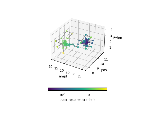
We can use this to see how the optimizer worked, color-coding each point by the statistic (using a log-normalized scale as we go from \(\gt 2000\) to \(\sim 30\)):
>>> fig, ax = plt.subplots(subplot_kw={"projection": "3d"})
>>> vmin = store['stat'].min()
>>> vmax = store['stat'].max()
>>> norm = colors.LogNorm(vmin=vmin, vmax=vmax)
>>> ax.plot(store['ampl'], store['pos'], store['fwhm'], c='k', alpha=0.4)
>>> scatter = ax.scatter(store['ampl'], store['pos'], store['fwhm'],
...                      c=store['stat'], norm=norm)
>>> ax.set_xlabel('ampl')
>>> ax.set_ylabel('pos')
>>> ax.set_zlabel('fwhm')
>>> cbar = fig.colorbar(scatter, shrink=0.5. orientation='horizontal')
>>> cbar.set_label('least-squares statistic')