Contributing to Sherpa development

Contributions to Sherpa - whether it be bug reports, documentation updates, or new code - are highly encouraged. Please report any problems or feature requests on github.

At present we do not have any explicit documentation on how to contribute to Sherpa, but it is similar to other open-source packages such as AstroPy.

The developer documentation is also currently lacking.

To do code development, Sherpa needs to be installed from source so that tests can run locally and the documentation can be build locally to test out any additions to code or docs. Building from source describes several ways to build Sherpa from source, but one particularly comfortable way is described in detail in the next section.

Pull requests

We welcome pull requests on github.

For each pull request, a set of continuous integration tests is run automatically, including a build of the documentation on readthedocs.

Skip the continuous integration

Sometimes a PR is still in development and known to fail the tests or simply does not touch any code, because it only modifies docstrings and the documentation. In that case, [skip ci] can be added to the commit message to prevent running the github actions tests to save time, energy, and limited resources.

Run tests locally

Before you issue a pull request, we ask to run the test suite locally. Assuming everything is set up to install Sherpa from source, it can be installed in development mode with pip:

pip install -e .

“Development mode” means that the tests will pick up changes in the Python source files without running pip again (which can take some time). Only if you change the C++ code, you will have to explicitly run the installation again to see the changes in the tests. After the installation, pytest can run all the tests. In the sherpa root directory call:

pytest

pytest supports a number of options which are detailed in the pytest documentation. A particularly useful option is to run only the tests in a specific file. For example, if you changed the code and the tests in the sherpa.astro.ui module, one might expect tests for this module to be the most likely to fail:

pytest sherpa/astro/ui/tests/test_astro_ui.py

Once everything looks good, you can do a final run of the entire test suite. A second option useful for develoment is --pdb which drops into the interactive Python debugger when a test fails so that you can move up and down the stack and inspect the value of individual variables.

The test suite can be sped up by running tests in parallel. After installing the pytest-xdist module (pip install pytest-xdist), tests can be run in parallel on several cores:

pytest -n auto

will autoselect the number of cores, an explicit number can also be given (pytest -n 4). Note that if you have DS9 and XPA installed then it is possible that the DS9 tests may fail when running tests in parallel (since multiple tests can end up over-writing the DS9 data before it can be checked).

Test coverage can be included as part of the tests by installing the coverage (pip install coverage) and pytest-cov packages (pip install pytest-cov). Adding the --cov=sherpa option to the test run allows us to generate a coverage report after that:

pytest --cov=sherpa
coverage html -d report

The report is in report/index.html, which links to individual files and shows exactly which lines were excuted while running the tests.

Run doctests locally

If doctestplus is installed (and it probably is because it’s part of sphinx-astropy, which is required to build the documentation locally), examples in the documentation are run automatically. This serves two purposes:

it ensure that the examples we give are actually correct and match the code,

and it acts as additional tests of the Sherpa code base.

The doctest_norecursedirs setting in the pytests.ini file is used to exclude files which can not be tested. This is generally because the examples were written before doctestplus support was added, and so they need to be re-worked, or there is too much extra set-up required that would make the examples hard-to follow. The file should be removed from this list when it has been updated to allow testing with doctestplus.

During development, you can run doctestplus on individual files like so (the option to use depends on whether it is a Python or reStructuredText file):

pytest --doctest-plus sherpa/astro/data.py
pytest --doctest-plus sherpa/data.py
pytest --doctest-rst docs/quick.rst
pytest --doctest-rst docs/evaluation/combine.rst

If you fix examples to pass these tests, remove them from the exclusion list in pytest.ini! The goal is to eventually pass on all files.

Some doctests (in the documentation or in the docstrings of individual functions) load data files. Those datafiles can be found in the sherpa-test-data directory as explained in the description of the development build. There is a conftest.py file in the sherpa/docs directory and in the sherpa/sherpa directory that sets up a pytest fixture to define a variable called data_dir which points to this directory. That way, we do not need to clutter the example with long directory names, but the sherpa-test-data directory has to be present as a submodule to successfully pass all doctests.

How do I …

Install from source in conda

Conda can be used to install all the dependencies for Sherpa, including XSPEC.

conda create -n sherpaciao -c https://cxc.cfa.harvard.edu/conda/ciao -c conda-forge ds9 astropy ciao
conda install -n sherpaciao --only-deps -c https://cxc.cfa.harvard.edu/conda/ciao -c conda-forge sherpa
conda activate sherpaciao

The first line installs the full CIAO release and astropy, required for building and running tests locally.

If you want to also build the documentation then add (after you have activated the environment):

conda install pandoc
pip install sphinx graphviz sphinx-astropy sphinx_rtd_theme nbsphinx ipykernel

Note

Sherpa can be configured to use crates (from CIAO) or astropy for it’s I/O backend by changing the contents of the file .sherpa-standalone.rc in your home directory. This file can be found, once CIAO is installed, by using the get_config routine:

% python -c 'import sherpa; print(sherpa.get_config())'
/home/happysherpauser/.sherpa-standalone.rc

If Sherpa was installed as part of CIAO then the file will be called .sherpa.rc.

The io_pkg line in this file can be changed to select crates rather than pyfits which would mean that astropy does not need to be installed (although it would be needed to build the documentation).

As described in Building from source, the file setup.cfg in the root directory of the sherpa source needs to be modified to configure the build. This is particularly easy in this setup, where all external dependencies are installed in conda and the enviroment variable ASCDS_INSTALL (or CONDA_PREFIX, which has the same value) can be used. For most cases, the scripts/use_ciao_config script can be used:

% ./scripts/use_ciao_config
Found XSPEC version: 12.12.0
Updating setup.cfg
% git diff setup.cfg
...

Otherwise the file can be edited manually. First find out what XSPEC version is present with:

% conda list xspec-modelsonly --json | grep version
    "version": "12.12.0"

then change the setup.cfg to change the following lines, noting that the ${ASCDS_INSTALL} environment variable must be replaced by its actual value, and the xspec_version line should be updated to match the output above:

bdist_wheel = sherpa_config xspec_config bdist_wheel

install_dir=${ASCDS_INSTALL}

configure=None

disable-group=True
disable-stk=True

fftw=local
fftw-include_dirs=${ASCDS_INSTALL}/include
fftw-lib-dirs=${ASCDS_INSTALL}/lib
fftw-libraries=fftw3

region=local
region-include_dirs=${ASCDS_INSTALL}/include
region-lib-dirs=${ASCDS_INSTALL}/lib
region-libraries=region ascdm
region-use-cxc-parser=True

wcs=local
wcs-include-dirs=${ASCDS_INSTALL}/include
wcs-lib-dirs=${ASCDS_INSTALL}/lib
wcs-libraries=wcs

with-xspec=True
xspec_version = 12.12.0
xspec_lib_dirs = ${ASCDS_INSTALL}/lib
xspec_include_dirs = ${ASCDS_INSTALL}/include

Note

The XSPEC version may include the patch level, such as 12.12.0e, and this can be included in the configuration file.

To avoid accidentially commiting the modified setup.cfg into git, the file can be marked as “assumed unchanged”.

git update-index --assume-unchanged setup.cfg

After these steps, Sherpa can be built from source:

pip install .

Warning

Just like in the case of a normal source install, when building Sherpa on recent versions of macOS within a conda environment, the following environment variable must be set:

export PYTHON_LDFLAGS=' '

That is, the variable is set to a space, not the empty string.

Warning

This is not guaranteed to build Sherpa in exactly the same manner as used by CIAO. Please create an issue if this causes problems.

Update the Zenodo citation information

The sherpa.citation() function returns citation information taken from the Zenodo records for Sherpa. It can query the Zenodo API, but it also contains a list of known releases in the sherpa._get_citation_hardcoded routine. To add to this list (for when there’s been a new release), run the scripts/make_zenodo_release.py script with the version number and add the screen output to the list in _get_citation_hardcoded.

For example, using release 4.12.2 would create (the author list has been simplified):

% ./scripts/make_zenodo_release.py 4.12.2
    add(version='4.12.2', title='sherpa/sherpa: Sherpa 4.12.2',
        date=todate(2020, 10, 27),
        authors=['Doug Burke', 'Omar Laurino', ... 'Todd'],
        idval='4141888')

Add a new notebook

The easiest way to add a new notebook to the documentation is to add it to the desired location in the docs/ tree and add it to the table of contents. If you want to place the notebook into the top-level notebooks/ directory and also have it included in the documentation then add an entry to the notebooks/nbmapping.dat file, which is a tab-separated text file listing the name of the notebook and the location in the docs/ directory structure that it should be copied to. The docs/conf.py file will ensure it is copied (if necessary) when building the documentation. The location of the documentation version must be added to the .gitignore file (see the section near the end) to make sure it does not accidentally get added.

If the notebook is not placed in notebooks/ then the nbsphinx_prolog setting in docs/conf.py will need updating. This sets the text used to indicate the link to the notebook on the Sherpa repository.

At present we require that the notebook be fully evaluated as we do not run the notebooks while building the documentation.

Add a new test option?

The sherpa/conftest.py file contains general-purpose testing routines, fixtures, and configuration support for the test suite. To add a new command-line option:

add to the pytest_addoption routine, to add the option;
add to pytest_collection_modifyitems if the option adds a new mark;
and add support in pytest_configure, such as registering a new mark.

Update the XSPEC bindings?

The sherpa.astro.xspec module currently supports XSPEC versions 12.13.1, 12.13.0, 12.12.1, and 12.12.0. It may build against newer versions, but if it does it will not provide access to any new models in the release. The following sections of the XSPEC manual should be reviewed: Appendix F: Using the XSPEC Models Library in Other Programs, and Appendix C: Adding Models to XSPEC.

Checking against a previous XSPEC version

If you have a version of Sherpa compiled with a previous XSPEC version then you can use two helper scripts:

scripts/check_xspec_update.py

This will compare the supported XSPEC model classes to those from a model.dat file, and report on the needed changes.
scripts/add_xspec_model.py

This will report the basic code needed to be added to both the compiled code (sherpa/astro/xspec/src/_xspec.cc) and Python (sherpa/astro/xspec/__init__.py). Note that it does not deal with conditional compilation, the need to add a decorator to the Python class, or missing documentation for the class.

These routines are designed to simplify the process but are not guaranteed to handle all cases (as the model.dat file syntax is not strongly specified).

As an example of their use, the following output is from before XSPEC 12.12.0 (released in HEASOFT 6.29) support was added:

% ./scripts/check_xspec_update.py ~/local/heasoft-6.29/spectral/manager/model.dat | grep support
We do not support grbjet (Add; xsgrbjet)
We do not support smaug (Add; xsmaug)
We do not support vvwdem (Add; vvwDem)
We do not support vwdem (Add; vwDem)
We do not support wdem (Add; wDem)
We do not support zxipab (Mul; zxipab)
We do not support pileup (Acn; pileup)

Note

There can be other output due to parameter-value changes which are also important to review but this is just focussing on the list of models that could be added to sherpa.astro.xspec.

The screen output may differ slightly from that shown above, such as including the interface used by the model (e.g. C, C++, FORTRAN).

The code needed to add support for the wdem module can be found with:

% ./scripts/add_xspec_model.py ~/local/heasoft-6.29/spectral/manager/model.dat wdem
# C++ code for sherpa/astro/xspec/src/_xspec.cc

// Defines

extern "C" {

}

// Wrapper

static PyMethodDef Wrappers[] = {
  XSPECMODELFCT_C_NORM(C_wDem, 8),
  { NULL, NULL, 0, NULL }
}


# Python code for sherpa/astro/xspec/__init__.py


class XSwdem(XSAdditiveModel):
    """XSPEC AdditiveModel: wdem

    Parameters
    ----------
    Tmax
    beta
    p
    nH
    abundanc
    Redshift
    switch
    norm

    """
    _calc = _models.C_wDem

    def __init__(self, name='wdem'):
        self.Tmax = Parameter(name, 'Tmax', 1.0, min=0.01, max=10.0, hard_min=0.01, hard_max=20.0, units='keV')
        self.beta = Parameter(name, 'beta', 0.1, min=0.01, max=1.0, hard_min=0.01, hard_max=1.0)
        self.p = Parameter(name, 'p', 0.25, min=-1.0, max=10.0, hard_min=-1.0, hard_max=10.0)
        self.nH = Parameter(name, 'nH', 1.0, min=1e-05, max=1e+19, hard_min=1e-06, hard_max=1e+20, frozen=True, units='cm^-3')
        self.abundanc = Parameter(name, 'abundanc', 1.0, min=0.0, max=10.0, hard_min=0.0, hard_max=10.0, frozen=True)
        self.Redshift = Parameter(name, 'Redshift', 0.0, min=-0.999, max=10.0, hard_min=-0.999, hard_max=10.0, frozen=True)
        self.switch = Parameter(name, '_switch', 2, alwaysfrozen=True)
        self.norm = Parameter(name, 'norm', 1.0, min=0.0, max=1e+24, hard_min=0.0, hard_max=1e+24)
        XSAdditiveModel.__init__(self, name, (self.Tmax,self.beta,self.p,self.nH,self.abundanc,self.Redshift,self.switch,self.norm))

This code then can then be added to sherpa/astro/xspec/src/_xspec.cc and sherpa/astro/xspec/__init__.py and then refined so that the tests pass.

Updating the code

The following steps are needed to update to a newer version, and assume that you have the new version of XSPEC, or its model library, available.

Add a new version define in helpers/xspec_config.py.

Current version: helpers/xspec_config.py.

When adding support for XSPEC 12.12.1, the top-level SUPPORTED_VERSIONS list was changed to include the triple (12, 12, 1):
```
SUPPORTED_VERSIONS = [(12, 12, 0), (12, 12, 1)]
```
This list is used to select which functions to include when compiling the C++ interface code. For reference, the defines are named XSPEC_<a>_<b>_<c> for each supported XSPEC release <a>.<b>.<c> (the XSPEC patch level is not included).

Note

The Sherpa build system requires that the user indicate the version of XSPEC being used, via the xspec_config.xspec_version setting in their setup.cfg file (as attempts to identify this value automatically were not successful). This version is the value used in the checks in helpers/xspec_config.py.
Attempt to build the XSPEC interface with:
```
pip install -e . --verbose
```
This requires that the xspec_config section of the setup.cfg file has been set up correctly for the new XSPEC release. The exact settings depend on how XSPEC was built (e.g. model only or as a full application), and are described in the building XSPEC documentation. The most-common changes are that the version numbers of the CCfits, wcslib, and hdsp libraries need updating, and these can be checked by looking in $HEADAS/lib.

If the build succeeds, you can check that it has worked by directly importing the XSPEC module, such as with the following, which should print out the correct version:
```
python -c 'from sherpa.astro import xspec; print(xspec.get_xsversion())'
```
It may however fail, due to changes in the XSPEC interface (unfortunately, such changes are often not included in the release notes).
Identify changes in the XSPEC models.

Note

The scripts/check_xspec_update.py and scripts/add_xspec_model.py scripts can be used to automate some - but unfortunately not all - of this.

A new XSPEC release can add models, change parameter settings in existing models, change how a model is called, or even delete a model (the last case is rare, and may require a discussion on how to proceed). The XSPEC release notes page provides an overview, but the model.dat file - found in headas-<version>/Xspec/src/manager/model.dat (build) or $HEADAS/../spectral/manager/model.dat (install) - provides the details. It greatly simplifies things if you have a copy of this file from the previous XSPEC version, since then a command like:
```
diff heasoft-6.26.1/spectral/manager/model.dat heasoft-6.27/spectral/manager/model.dat
```
will tell you the differences (this example was for XSPEC 12.11.0, please adjust as appropriate). If you do not have the previous version then the release notes will tell you which models to look for in the model.dat file.

The model.dat is an ASCII file which is described in Appendix C: Adding Models to XSPEC of the XSPEC manual. The Sherpa interface to XSPEC only supports models labelled as add, mul, and con (additive, multiplicative, and convolution, respectively).

Each model is represented by a set of consecutive lines in the file, and as of XSPEC 12.11.0, the file begins with:
```
% head -5 heasoft-6.27/Xspec/src/manager/model.dat
agauss         2   0.         1.e20          C_agauss  add  0
LineE   A      10.0   0.      0.      1.e6      1.e6      0.01
Sigma   A      1.0    0.      0.      1.e6      1.e6      0.01

agnsed        15   0.03       1.e20          agnsed    add  0
```
The important parts of the model definition are the first line, which give the XSPEC model name (first parameter), number of parameters (second parameter), two numbers which we ignore, the name of the function that evaluates the model, the type (e.g. add), and then 1 or more values which we ignore. Then there are lines which define the model parameters (the number match the second argument of the first line), and then one or more blank lines. In the output above we see that the XSPEC agauss model has 2 parameters, is an additive model provided by the C_agauss function, and that the parameters are LineE and Sigma. The agnsed model is then defined (which uses the agnsed routines), but its 15 parameters have been cut off from the output.

The parameter lines will mostly look like this: parameter name, unit string (is often " "), the default value, the hard and then soft minimum, then the soft ahd hard maximum, and then a value used by the XSPEC optimiser, but we only care about if it is negative (which indicates that the parameter should be frozen by default). The other common variant is the “flag” parameter - that is, a parameter that should never be thawed in a fit - which is indicated by starting the parameter name with a $ symbol (although the documentation says these should only be followed by a single value, you’ll see a variety of formats in the model.dat file). These parameters are marked by setting the alwaysfrozen argument of the Parameter constructor to True. Another option is the “scale” parameter, which is labelled with a * prefix, and these are treated as normal parameter values.

Note

The examples below may refer to XSPEC versions we no-longer support.
1. sherpa/astro/xspec/src/_xspec.cc
  
  Current version: sherpa/astro/xspec/src/_xspec.cc.
  
  New functions are added to the XspecMethods array, using macros defined in sherpa/include/sherpa/astro/xspec_extension.hh, and should be surrounded by a pre-processor check for the version symbol added to helpers/xspec_config.py.
  
  As an example:
```
#ifdef XSPEC_12_12_0
  XSPECMODELFCT_C_NORM( C_wDem, 8 )
#endif
```
  adds support for the C_wDem function, but only for XSPEC 12.12.0 and later. Note that the symbol name used here is not the XSPEC model name (the first argument of the model definition from model.dat), but the function name (the fifth argument of the model definition):
```
% grep C_wDem $HEADAS/../spectral/manager/model.dat
wdem          7  0.         1.e20           C_wDem   add  0
```
  Some models have changed the name of the function over time, so the pre-processor directive may need to be more complex, such as the following (although now we no-longer support XSPEC 12.10.0 this particular example has been removed from the code):
```
#ifdef XSPEC_12_10_0
  XSPECMODELFCT_C_NORM( C_nsmaxg, 6 ),
#else
  XSPECMODELFCT_NORM( nsmaxg, 6 ),
#endif
```
  The remaining pieces are the choice of macro (e.g. XSPECMODELFCT_NORM or XSPECMODELFCT_C_NORM) and the value for the second argument. The macro depends on the model type and the name of the function (which defines the interface that XSPEC provides for the model, such as single- or double- precision, and Fortran- or C- style linking). Additive models use the suffix _NORM and convolution models use the suffix _CON. Model functions which begin with C_ use the _C variant, while those which begin with c_ currently require treating them as if they have no prefix.
  
  The numeric argument to the template defines the number of parameters supported by the model once in Sherpa, and should equal the value given in the model.dat file for multiplicative and convolution style models, and one larger than this for additive models (i.e. those which use a macro that ends in _NORM).
  
  As an example, the following three models from model.dat:
```
apec           3  0.         1.e20           C_apec    add  0
phabs          1  0.03       1.e20           xsphab    mul  0
gsmooth        2  0.         1.e20           C_gsmooth    con  0
```
  are encoded as (ignoring any pre-processor directives):
```
XSPECMODELFCT_C_NORM( C_apec, 4 ),
XSPECMODELFCT( xsphab, 1 ),
XSPECMODELFCT_CON(C_gsmooth, 2),
```
  Those models that do not use the _C version of the macro (or, for convolution-style models, have to use XSPECMODELFCT_CON_F77), also have to declare the function within the extern "C" {} block. For FORTRAN models, the declaration should look like (replacing func with the function name, and note the trailing underscore):
```
xsf77Call func_;
```
  and for model functions called c_func, the prefixless version should be declared as:
```
xsccCall func;
```
  If you are unsure, do not add a declaration and then try to build Sherpa: the compiler should fail with an indication of what symbol names are missing.
  
  Note
  
  Ideally we would have a sensible ordering for the declarations in this file, but at present it is ad-hoc.
2. sherpa/astro/xspec/__init__.py
  
  Current version: sherpa/astro/xspec/__init__.py.
  
  This is where the Python classes are added for additive and multiplicative models. The code additions are defined by the model and parameter specifications from the model.dat file, and the existing classes should be used for inspiration. The model class should be called XS<name>, where <name> is the XSPEC model name, and the name argument to its constructor be set to the XSPEC model name.
  
  The two main issues are:
  - Documentation: there is no machine-readable version of the text, and so the documentation for the XSPEC model is used for inspiration.
    
    The idea is to provide minimal documentation, such as the model name and parameter descriptions, and then to point users to the XSPEC model page for more information.
    
    One wrinkle is that the XSPEC manual does not provide a stable URI for a model (as it can change with XSPEC version). However, it appears that you can use the following pattern:
    
    https://heasarc.gsfc.nasa.gov/xanadu/xspec/manual/XSmodel<Name>.html
    
    where <Name> is the capitalised version of the model name (e.g. Agnsed).
  - Models that are not in older versions of XSPEC should be marked with the version_at_least decorator (giving it the minimum supported XSPEC version as a string), and the function (added to _xspec.cc) is specified as a string using the __function__ attribute. The sherpa.astro.xspec.utils.ModelMeta metaclass performs a runtime check to ensure that the model can be used.
    
    For example (from when XSPEC 12.9.0 was still supported):
    __function__ = "C_apec" if equal_or_greater_than("12.9.1") else "xsaped"
3. sherpa/astro/xspec/tests/test_xspec.py
  
  Current version: sherpa/astro/xspec/tests/test_xspec.py.
  
  The XSPEC_MODELS_COUNT version should be increased by the number of models classes added to __init__.py.
  
  Additive and multiplicative models will be run as part of the test suite - using a simple test which runs on a default grid and uses the default parameter values - whereas convolution models are not (since their pre-conditions are harder to set up automatically).
4. docs/model_classes/astro_xspec.rst
  
  Current version: docs/model_classes/astro_xspec.rst.
  
  New models should be added to both the Classes rubric - sorted by addtive and then multiplicative models, using an alphabetical sorting - and to the appropriate inheritance-diagram rule.
Documentation updates

The docs/indices.rst file should be updated to add the new version to the list of supported versions, under the XSPEC term, and docs/developer/index.rst also lists the supported versions (Update the XSPEC bindings?). The installation page docs/install.rst should be updated to add an entry for the setup.cfg changes in XSPEC.

The sherpa/astro/xspec/__init__.py file also lists the supported XSPEC versions.

Never forget to update the year of the copyright notice?

Git offers pre-commit hooks that can do file checks for you before a commit is executed. The script in scripts/pre-commit will check if the copyright notice in any of the files in the current commit must be updated and, if so, add the current year to the copyright notice and abort the commit so that you can manually check before commiting again.

To use this opt-in functionality, simply copy the file to the appropriate location:

cp scripts/pre-commit .git/hooks

Notes

Notes on the design and changes to Sherpa.

N-dimensional data and models

Models and data objects are designed to work with flattened arrays, so a 1D dataset has x and y for the independent and dependent axes, and a 2D dataset will have x0, x1, and y values, with each value stored as a 1D ndarray. This makes it easy to deal with filters and sparse or irregularly-placed grids.

>>> from sherpa.data import Data1D, Data1DInt, Data2D

As examples, we have a one-dimensional dataset with data values (dependent axis, y) of 2.3, 13.2, and -4.3 corresponding to the independent axis (x) values of 1, 2, and 5:

>>> d1 = Data1D("ex1", [1, 2, 5], [2.3, 13.2, -4.3])

An “integrated” one-dimensional dataset for the independent axis bins 23-44, 45-50, 50-53, and 55-57, with data values of 12, 14, 2, and 22 looks like this:

>>> d2 = Data1DInt("ex2", [23, 45, 50, 55], [44, 50, 53, 57], [12, 14, 2, 22])

An irregularly-gridded 2D dataset, with points at (-200, -200), (-200, 0), (0, 0), (200, -100), and (200, 150) can be created with:

>>> d3 = Data2D("ex3", [-200, -200, 0, 200, 200], [-200, 0, 0, -100, 150],
... [12, 15, 23, 45, -2])

A regularly-gridded 2D dataset can be created, but note that the arguments must be flattened:

>>> import numpy as np
>>> x1, x0 = np.mgrid[20:30:2, 5:20:2]
>>> shp = x0.shape
>>> y = np.sqrt((x0 - 10)**2 + (x1 - 31)**2)
>>> x0 = x0.flatten()
>>> x1 = x1.flatten()
>>> y = y.flatten()
>>> d4 = Data2D("ex4", x0, x1, y, shape=shp)

The dimensionality of models

Originally the Sherpa model class did not enforce any requirement on the models, so it was possible to combine 1D and 2D models, even though the results are unlikely to make sense. With the start of the regrid support, added in PR #469, the class hierarchy included 1D- and 2D- specific classes, but there was still no check on model expressions. This section describes the current way that models are checked:

the sherpa.models.model.Model class defines a sherpa.models.model.Model.ndim attribute, which is set to None by default.
the sherpa.models.model.RegriddableModel1D and sherpa.models.model.RegriddableModel2D classes set this attribute to 1 or 2, respectively (most user-callable classes are derived from one of these two classes).
the sherpa.models.model.CompositeModel class checks the ndim attribute for the components it is given (the parts argument) and checks that they all have the same ndim value (ignoring those models whose dimensionality is set to None). If there is a mis-match then a sherpa.utils.err.ModelErr is raised.
as described below, the dimensions of data and model can be compared.

An alternative approach would have been to introduce 1D and 2D specific classes, from which all models derive, and then require the parent classes to match. This was not attempted as it would require significantly-larger changes to Sherpa (but this change could still be made in the future).

The data class

Prior to Sherpa 4.14.1, the Data object did not have many explicit checks on the data it was sent, instead relying on checks when the data was used. Now, validation checks are done when fields are changed, rather than when the data is used. This has been done primarily by marking field accessors as property attributes, so that they can apply the validation checks when the field is changed. The intention is not to catch all possible problems, but to cover the obvious cases.

Data dimensionality

Data objects have a ndim field, which is used to ensure that the model and data dimensions match when using the eval_model and eval_model_to_fit methods.

The size of a data object

The size field describes the size of a data object, that is the number of individual elements. Once a data object has its size set it can not be changed (this is new to Sherpa 4.14.1, as in previous versions you could change fields to any size). This field can also be accessed using len, with it returning 0 when no data has been set.

Point versus Integrated

There is currently no easy way to identify whether a data object requires integrated (low and high edges) or point axes (the coordinate at which to evaluate the model).

Handling the independent axis

Checks have been added in Sherpa 4.14.1 to ensure that the correct number of arrays are used when setting the independent axis: that is, a Data1D object uses (x,), Data1DInt uses (lo, hi), and Data2D uses (x0, x1). Note that the arguement is expected to be a tuple, even in the Data1D case, and that the individual components are checked to ensure they have the same size.

The handling of the independent axis is mediated by a “Data Space” object (DataSpaceND, DataSpace1D, IntegratedDataSpace1D, DataSpace2D, and IntegratedDataSpace2D) which is handled by the _init_data_space and _check_data_space methods of the Data class.

To ensure that any filter remains valid, the independent axis is marked as read-only. The only way to change a value is to change the whole independent axis, in which case the code recognizes that the filter - whether just the mask attribute or also any region filter for the DataIMG case - has to be cleared.

Validation

Fields are converted to ndarray - if not None - and then checked to see if they are 1D and have the correct size. Some fields may have extra checks, such as the grouping and quality columns for PHA data which are converted to integer values.

One example of incomplete validation is that the bin_lo and bin_hi fields are not checked to ensure that both are set, or that they are in descending order, that the bin_hi value is always larger than the correspondnig bin_lo value, or that there are no overlapping bins.

Error messages

Errors are generally raised as DataErr exceptions, although there are cases when a ValueError or TypeError will be raised. The aim is to provide some context in the message, such as:

>>> from sherpa.data import Data1D
>>> x = np.asarray([1, 2, 3])
>>> y = np.asarray([1, 2])
>>> data = Data1D('example', x, y)
Traceback (most recent call last):
...
sherpa.utils.err.DataErr: size mismatch between independent axis and y: 3 vs 2

and:

>>> data = Data1D('example', x, x + 10)
>>> data.apply_filter(y)
Traceback (most recent call last):
...
sherpa.utils.err.DataErr: size mismatch between data and array: 3 vs 2

For DataPHA objects, where some length checks have to allow either the full size (all channels) or just the filtered data, the error messages could explain that both are allowed, but this was felt to be overly complicated, so the filtered size will be used.

PHA Filtering

Filtering of a DataPHA object has four complications compared to Data1D objects:

the independent axis can be referred to in channel units (normally 1 to the maximum number of channels), energy units (e.g. 0.5 to 7 keV), or wavelength units (e.g. 20 to 22 Angstroms);
each channel has a width of 1, so channel filters - which are generally going to be integer values - map exactly, but each channel has a finite width in the derived units (that is, energy or wavelength) so multiple values will map to the same channel (e.g. a channel may map to the energy range of 0.4 to 0.5 keV, so any value >= 0.4 and < 0.5 will map to it);
the data can be dynamically grouped via the grouping attribute, normally set by methods like group_counts() and controlled by the group() method, which means that the desired filter, when mapped to channel units, is likely to end up partially overlapping the first and last groups, which means that notice(a, b) and ignore(None, a); ignore(b, None) are not guaranteed to select the same range;
and there is the concept of the quality array, which defines whether channels should either always be, or can temporarily be, ignored.

This means that a notice() or ignore() call has to convert from the units of the input - which is defined by the units attribute, changeable with set_analysis - to the “group number” which then gets sent to the _data_space attribute to track the filter.

One result is that the mask attribute will now depend on the grouping scheme. The get_mask method can be used to calculate a mask for all channels (e.g. the ungrouped data).

There are complications to this from the quality concept introduced by the OGIP grouping scheme, which I have not been able to fully trace through in the code.

Combining model expressions

Models can be combined in several ways (for models derived from the sherpa.models.model.ArithmeticModel class):

a unary operator, taking advantage of the __neg__ and __abs__ special methods of a class;
a binary operator, using the __add__, __sub__, __mul__, __div__, __floordiv__, __truediv__, __mod__ and __pow__ methods.

This allows models such as:

sherpa.models.basic.Polynom1D('continuum') + sherpa.models.basic.Gauss1D('line')

to be created, and relies on the sherpa.models.model.UnaryOpModel and sherpa.models.model.BinaryOpModel classes.

The BinaryOpModel class has special-case handling for values that are not a model expression (i.e. that do not derive from the ArithmeticModel class), such as:

32424.43 * sherpa.astro.xspec.XSpowerlaw('pl')

In this case the term 32424.43 is converted to an ArithmeticConstantModel instance and then combined with the remaining model instance (XSpowerlaw).

For those models that require the full set of elements, such as multiplication by a RMF or a convolution kernel, this requires creating a model that can “wrap” another model. The wrapping model will evaluate the wrapped model on the requested grid, and then apply any modifications. Examples include the sherpa.instrument.PSFModel class, which creates sherpa.instrument.ConvolutionModel instances, and the sherpa.astro.xspec.XSConvolutionKernel class, which creates sherpa.astro.xspec.XSConvolutionModel instances.

When combining models, BinaryOpModel (actually, this check is handled by the super class CompositeModel), this approach will ensure that the dimensions of the two expressions match. There are some models, such as TableModel and ArithmeticConstantModel, which do not have a ndim attribute (well, it is set to None); when combining components these are ignored, hence treated as having “any” dimension.

Plotting data using the UI layer

The plotting routines, such as plot_data() and plot_fit(), follow the same scheme:

The plot object is retrieved by the appropriate get_xxx_plot routine, such as get_data_plot() and get_fit_plot().
These get_xxx_plot calls retrieve the correct plot object - which is normally a sub-class of Plot or Histogram - from the session object.

Note

The naming of these objects in the Session object is rather hap-hazard and would benefit from a more-structured approach.

If the recalc argument is set then the prepare method of the plot object is called, along with the needed data, which depends on the plot type - e.g. sherpa.plot.DataPlot.prepare needs data and statistic objects and sherpa.plot.ModelPlot.prepare needs data and model objects (and a statistic class too but in this case it isn’t used).

Calls to other access other plot objects may be required, such as the fit plot requiring both data and model objects. It is also the place that specialised logic, such as selecting a histogram-style plot for Data1DInt data rather than the default plot style, is made.

These plot objects generally do not require a plotting backend, so they can be set and returned even without Matplotlib installed.
Once the plot object has been retrieved, is is sent to a plotting routine - sherpa.ui.utils.Session._plot() - which calls the plot method of the object, passing through the plot options. It is at this point that the plot backend is used to create the visualization (these settings are passed as **kwargs down to the plot backend routines).

The sherpa.astro.ui.utils.Session class adds a number of plot types and classes, as well as adds support for the DataPHA class to relevant plot commands, such as plot_model() and plot_fit(). This support complicates the interpretation of the model and fit types, as different plot types are used to represent the model when drawn directly (plot_model) and indirectly (plot_fit): these plot classes handle binning differently (that is, whether to apply the grouping from the source PHA dataset or use the native grid of the response).

There are two routines that return the preference settings: get_data_plot_prefs and get_model_plot_prefs. The idea for these is that they return the preference dictionary that the relevant classes use. However, with the move to per-dataset plot types (in particular Data1DInt and DataPHA). It is not entirely clear how well this scheme works.

The contour routines follow the same scheme, although there is a lot less specialization of these methods, which makes the implementation easier. For these plot objects the sherpa.ui.utils.Session._contour() method is used instead (and rather than have overplot we have overcontour as the argument).

The sherpa.ui.utils.Session.plot() and sherpa.ui.utils.Session.contour() methods allow multiple plots to be created by specifying the plot type as a list of argumemts. For example:

>>> s.plot('data', 'model', 'data', 2, 'model', 2)  

will create four plots, in a two-by-two grid, showing the data and model values for the default dataset and the dataset numbered 2. The implementation builds on top of the individual routines, by mapping the command value to the necessary get_xxx_plot or get_xxx_contour routine.

The image routines are conceptually the same, but the actual implementation is different, in that it uses a centralized routine to create the image objects rather than have the logic encoded in the relavant get_xxx_image routines. It is planned to update the image code to match the plot and contour routines. The main difference is that the image display is handled via XPA calls to an external DS9 application, rather than with direct calls to the plotting library.

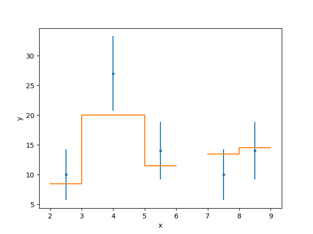
As an example, here I plot a “fit” for a Data1DInt dataset:

>>> from sherpa.ui.utils import Session
>>> from sherpa.data import Data1DInt
>>> from sherpa.models.basic import Const1D
>>> s = Session()
>>> xlo = [2, 3, 5, 7, 8]
>>> xhi = [3, 5, 6, 8, 9]
>>> y = [10, 27, 14, 10, 14]
>>> s.load_arrays(1, xlo, xhi, y, Data1DInt)
>>> mdl = Const1D('mdl')
>>> mdl.c0 = 6
>>> s.set_source(mdl)
>>> s.plot_fit()

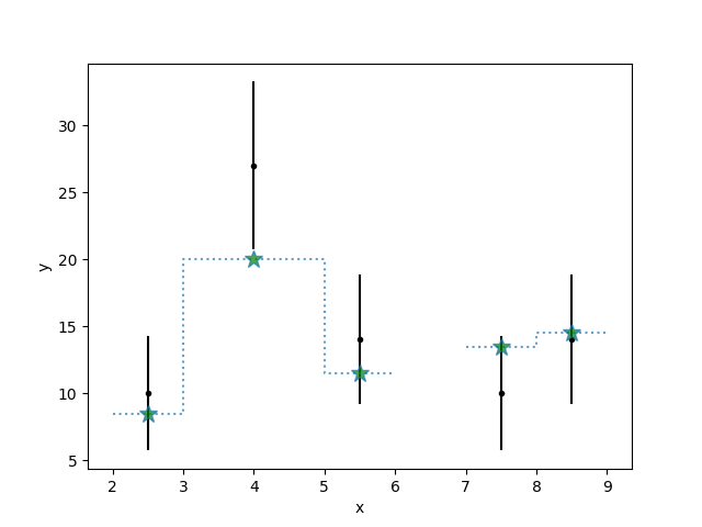
We can see how the Matplotlib-specific options are passed to the backend, using a combination of direct access, such as color='black', and via the preferences (the marker settings):

>>> s.plot_data(color='black')
>>> p = s.get_model_plot_prefs()
>>> p['marker'] = '*'
>>> p['markerfacecolor'] = 'green'
>>> p['markersize'] = 12
>>> s.plot_model(linestyle=':', alpha=0.7, overplot=True)

We can view the model plot object:

>>> plot = s.get_model_plot(recalc=False)
>>> print(type(plot))
<class 'sherpa.plot.ModelHistogramPlot'>
>>> print(plot)
xlo    = [2,3,5,7,8]
xhi    = [3,5,6,8,9]
y      = [ 6.,12., 6., 6., 6.]
xlabel = x
ylabel = y
title  = Model
histo_prefs = {'xerrorbars': False, 'yerrorbars': False, ..., 'linecolor': None}

Coordinate conversion for image data

The sherpa.data.Data2D class provides basic support for fitting models to two-dimensional data; that is, data with two independent axes (called “x0” and “x1” although they should be accessed via the indep attribute). The sherpa.astro.data.DataIMG class extends the 2D support to include the concept of a coordinate system, allowing the independent axis to be one of:

logical
image
world

where the aim is that the logical system refers to a pixel number (no coordinate system), image is a linear transform of the logical system, and world identifies a projection from the image system onto the celestial sphere. However, there is no requirement that this categorization holds as it depends on whether the optional sky and eqpos attributes are set when the DataIMG object is created.

Using a coordinate system directly

Note

It is expected that the DataIMG object is used with a rectangular grid of data and a shape attribute set up to describe the grid shape, as used in the next section, but it is not required, as shown here.

If the independent axes are known, and not calculated via a coordinate transform, then they can just be set when creating the DataIMG object, leaving the coord attribute set to logical.

>>> from sherpa.astro.data import DataIMG
>>> x0 = np.asarray([1000, 1200, 2000])
>>> x1 = np.asarray([-500, 500, -500])
>>> y = np.asarray([10, 200, 30])
>>> d = DataIMG("example", x0, x1, y)
>>> print(d)
name      = example
x0        = Int64[3]
x1        = Int64[3]
y         = Int64[3]
shape     = None
staterror = None
syserror  = None
sky       = None
eqpos     = None
coord     = logical

This can then be used to evaluate a two-dimensional model, such as Gauss2D:

>>> from sherpa.models.basic import Gauss2D
>>> mdl = Gauss2D()
>>> mdl.xpos = 1500
>>> mdl.ypos = -100
>>> mdl.fwhm = 1000
>>> mdl.ampl = 100
>>> print(mdl)
gauss2d
   Param        Type          Value          Min          Max      Units
   -----        ----          -----          ---          ---      -----
   gauss2d.fwhm thawed         1000  1.17549e-38  3.40282e+38
   gauss2d.xpos thawed         1500 -3.40282e+38  3.40282e+38
   gauss2d.ypos thawed         -100 -3.40282e+38  3.40282e+38
   gauss2d.ellip frozen            0            0        0.999
   gauss2d.theta frozen            0     -6.28319      6.28319    radians
   gauss2d.ampl thawed          100 -3.40282e+38  3.40282e+38
>>> d.eval_model(mdl)
array([32.08564744, 28.71745887, 32.08564744])

Attempting to change the coordinate system with set_coord will error out with a DataErr instance reporting that the data set does not specify a shape.

The shape attribute

The shape argument can be set when creating a DataIMG object to indicate that the data represents an “image”, that is a rectangular, contiguous, set of pixels. It is defined as (nx1, nx0), and so matches the ndarray shape attribute from NumPy. Operations that treat the dataset as a 2D grid often require that the shape attribute is set.

>>> x1, x0 = np.mgrid[1:4, 1:5]
>>> y2 = (x0 - 2.5)**2 + (x1 - 2)**2
>>> y = np.sqrt(y2)
>>> d = DataIMG('img', x0.flatten(), x1.flatten(),
...             y.flatten(), shape=y.shape)
>>> print(d)
name      = img
x0        = Int64[12]
x1        = Int64[12]
y         = Float64[12]
shape     = (3, 4)
staterror = None
syserror  = None
sky       = None
eqpos     = None
coord     = logical
>>> d.get_x0()
array([1, 2, 3, 4, 1, 2, 3, 4, 1, 2, 3, 4])
>>> d.get_x1()
array([1, 1, 1, 1, 2, 2, 2, 2, 3, 3, 3, 3])
>>> d.get_dep()
array([1.80277564, 1.11803399, 1.11803399, 1.80277564, 1.5       ,
       0.5       , 0.5       , 1.5       , 1.80277564, 1.11803399,
       1.11803399, 1.80277564])
>>> d.get_axes()
(array([1., 2., 3., 4.]), array([1., 2., 3.]))
>>> d.get_dims()
(4, 3)

Attempting to change the coordinate system with set_coord will error out with a DataErr instance reporting that the data set does not contain the required coordinate system.

Setting a coordinate system

The sherpa.astro.io.wcs.WCS class is used to add a coordinate system to an image. It has support for linear (translation and scale) and “wcs” - currently only tangent-plane projections are supported - conversions.

>>> from sherpa.astro.io.wcs import WCS
>>> sky = WCS("sky", "LINEAR", [1000,2000], [1, 1], [2, 2])
>>> x1, x0 = np.mgrid[1:3, 1:4]
>>> d = DataIMG("img", x0.flatten(), x1.flatten(), np.ones(x1.size), shape=x0.shape, sky=sky)
>>> print(d)
name      = img
x0        = Int64[6]
x1        = Int64[6]
y         = Float64[6]
shape     = (2, 3)
staterror = None
syserror  = None
sky       = sky
 crval    = [1000.,2000.]
 crpix    = [1.,1.]
 cdelt    = [2.,2.]
eqpos     = None
coord     = logical

With this we can change to the “physical” coordinate system, which represents the conversion sent to the sky argument, and so get the independent axis in the converted system with the set_coord method:

>>> d.get_axes()
(array([1., 2., 3.]), array([1., 2.]))
>>> d.set_coord("physical")
>>> d.get_axes()
(array([1000., 1002., 1004.]), array([2000., 2002.]))
>>> d.indep
(array([1000., 1002., 1004., 1000., 1002., 1004.]), array([2000., 2000., 2000., 2002., 2002., 2002.]))

It is possible to switch back to the original coordinate system (the arguments sent in as x0 and x1 when creating the object):

>>> d.set_coord("logical")
>>> d.indep
(array([1, 2, 3, 1, 2, 3]), array([1, 1, 1, 2, 2, 2]))

In Sherpa 4.14.0 and earlier, this conversion was handled by taking the current axes pair and applying the necessary WCS objects to create the selected coordinate system (that is, the argument to the set_coord call). This had the advantage of saving memory, as you only needed to retain the current pair of independent axes, but at the expense of losing fidelity when converting between the coordinate systems. This has been changed so that the original independent axes are now stored in the object, in the _orig_indep_axis attribute, and this is now used whenever the coordinate system is changed. This does increase the memory size of a DataIMG object, and makes it harder to load in picked files created with an old Sherpa version (the code will do its best to create the necessary information but it is not guaranteed to work well in all cases).