Notebook support in Sherpa
A number of objects have been updated to support HTML output when displayed in a Jupyter notebook. Let’s take a quick tour!
Data1D, Data1DInt, and Data2D
First we have the data objects:
[1]:
import numpy as np

from sherpa.data import Data1D, Data1DInt, Data2D

x = np.arange(100, 200, 20)
y = [120, 240, 30, 95, 130]

d1 = Data1D('oned', x, y)
d1i = Data1DInt('onedint', x[:-1], x[1:], y[:-1])

x0 = [150, 250, 100]
x1 = [250, 200, 200]
y2 = [50, 40, 70]
d2 = Data2D('twod', x0, x1, y2)
Each can be displayed with print, which shows a textual representation of attribute and values:
[2]:
print(d1)
name      = oned
x         = Int64[5]
y         = Int64[5]
staterror = None
syserror  = None
Or they can be displayed as-is which, in a Jupyter notebook, will display either a plot or a HTML table. The Data1D and Data1DInt classes will display a plot (if the pylab plotting backend is selected), and the Data2D class a table.
[3]:
d1
[3]:
Data1D Plot
[4]:
print(d1i)
name      = onedint
xlo       = Int64[4]
xhi       = Int64[4]
y         = Int64[4]
staterror = None
syserror  = None
[5]:
d1i
[5]:
Data1DInt Plot
As mentioned, the Data2D class just gets a fancy HTML table but no plot:
[6]:
print(d2)
name      = twod
x0        = Int64[3]
x1        = Int64[3]
y         = Int64[3]
shape     = None
staterror = None
syserror  = None
[7]:
d2
[7]:
Data2D Summary (5)
DataPHA, DataARF, and DataRMF
The Astronomy-specific PHA, ARF, and RMF data classes can also be displayed. These (when you have pylab selected) display both the data and a table of information.
[8]:
from sherpa.astro import io

pha = io.read_pha('../sherpa-test-data/sherpatest/9774.pi')
arf = io.read_arf('../sherpa-test-data/sherpatest/9774.arf')
rmf = io.read_rmf('../sherpa-test-data/sherpatest/9774.rmf')
read ARF file ../sherpa-test-data/sherpatest/9774.arf
read RMF file ../sherpa-test-data/sherpatest/9774.rmf
read background file ../sherpa-test-data/sherpatest/9774_bg.pi
[9]:
print(pha)
name           = ../sherpa-test-data/sherpatest/9774.pi
channel        = Float64[1024]
counts         = Float64[1024]
staterror      = None
syserror       = None
grouping       = None
quality        = None
exposure       = 75141.227687398
backscal       = 4.3513325252917e-07
areascal       = 1.0
grouped        = False
subtracted     = False
units          = energy
rate           = True
plot_fac       = 0
response_ids   = [1]
background_ids = [1]
[10]:
pha
[10]:
PHA Plot
Summary (7)
Metadata (10)
The PHA object will change the display based on the data - that is, if you change the filtering and grouping you will see a different plot, and the table will also change:
[11]:
pha.notice(0.3, 7)
pha.group_counts(20, tabStops=~pha.mask)

pha
[11]:
PHA Plot
Summary (8)
Metadata (10)
It will also change if you change the analysis setting:
[12]:
pha.set_analysis('wave')

pha
[12]:
PHA Plot
Summary (8)
Metadata (10)
The ARF and RMF objects do not change based on their settings:
[13]:
print(arf)
name     = ../sherpa-test-data/sherpatest/9774.arf
energ_lo = Float64[1078]
energ_hi = Float64[1078]
specresp = Float64[1078]
exposure = 75141.231099099
ethresh  = 1e-10
[14]:
arf
[14]:
ARF Plot
Summary (5)
Metadata (6)
[15]:
print(rmf)
name     = ../sherpa-test-data/sherpatest/9774.rmf
energ_lo = Float64[1078]
energ_hi = Float64[1078]
n_grp    = UInt64[1078]
f_chan   = UInt64[1481]
n_chan   = UInt64[1481]
matrix   = Float64[438482]
e_min    = Float64[1024]
e_max    = Float64[1024]
detchans = 1024
offset   = 1
ethresh  = 1e-10
For the RMF, five energies are selected that span the response of the instrument, and the response to these monochromatic energies are displayed.
[16]:
rmf
[16]:
RMF Plot
Summary (5)
Metadata (6)
DataIMG
For images with little metadata, and no WCS information, we just get an image:
[17]:
img = io.read_image('../sherpa-test-data/sherpatest/img.fits')
[18]:
img
[18]:
DataIMG Plot
If the image contains WCS information, or some basic metadata, then we will get extra tables (unfortunately this test image doesn’t display particularly wonderfully as the source is faint!).
[19]:
img2 = io.read_image('../sherpa-test-data/sherpatest/acisf08478_000N001_r0043_regevt3_srcimg.fits')

img2
[19]:
DataIMG Plot
Coordinates: physical (3)
Coordinates: world (6)
Metadata (6)
As with the PHA object, we can change the display slightly, such as changing the coord setting and spatially filtering the data:
[20]:
img2.set_coord('physical')
img2.notice2d('circle(3150, 4520, 20)')

img2
[20]:
DataIMG Plot
Coordinates: physical (3)
Coordinates: world (6)
Metadata (6)
Models and parameters
Models and parameters can also be displayed directly as HTML tables, mirroring their print output.
[21]:
from sherpa.models.basic import Gauss2D, Const2D

mgauss = Gauss2D()
mconst = Const2D()

mgauss.xpos = 3150
mgauss.ypos = 4520

mdl = mgauss + mconst
We can compare the model output (this also works with a single component, such as mgauss and mconst):
[22]:
print(mdl)
gauss2d + const2d
   Param        Type          Value          Min          Max      Units
   -----        ----          -----          ---          ---      -----
   gauss2d.fwhm thawed           10  1.17549e-38  3.40282e+38
   gauss2d.xpos thawed         3150 -3.40282e+38  3.40282e+38
   gauss2d.ypos thawed         4520 -3.40282e+38  3.40282e+38
   gauss2d.ellip frozen            0            0        0.999
   gauss2d.theta frozen            0     -6.28319      6.28319    radians
   gauss2d.ampl thawed            1 -3.40282e+38  3.40282e+38
   const2d.c0   thawed            1 -3.40282e+38  3.40282e+38
[23]:
mdl
[23]:
Model
| Component | Parameter | Thawed | Value | Min | Max | Units |
|---|---|---|---|---|---|---|
| gauss2d | fwhm | 10.0 | TINY | MAX | ||
| xpos | 3150.0 | -MAX | MAX | |||
| ypos | 4520.0 | -MAX | MAX | |||
| ellip | 0.0 | 0.0 | 0.999 | |||
| theta | 0.0 | -2π | 2π | radians | ||
| ampl | 1.0 | -MAX | MAX | |||
| const2d | c0 | 1.0 | -MAX | MAX |
We can have a display for parameters (I chose this model since we can see the minimum and maximum columns get displayed as units of \(\pi\) in the notebook-display version):
[24]:
print(mgauss.theta)
val         = 0.0
min         = -6.283185307179586
max         = 6.283185307179586
units       = radians
frozen      = True
link        = None
default_val = 0.0
default_min = -6.283185307179586
default_max = 6.283185307179586
[25]:
mgauss.theta
[25]:
Parameter
| Component | Parameter | Thawed | Value | Min | Max | Units |
|---|---|---|---|---|---|---|
| gauss2d | theta | 0.0 | -2π | 2π | radians |
Fitting data
Various objects related to fitting will also display in Jupyter notebooks. I fit a simple model (the model we just created, in fact) to the last image we were looking at. For this example I use the sherpa.astro.ui layer to fit, rather than creating the fit object manually.
[26]:
from sherpa.astro import ui

ui.set_data(img2)
ui.set_source(mdl)

ui.set_stat('cash')
ui.set_method('simplex')
WARNING: imaging routines will not be available,
failed to import sherpa.image.ds9_backend due to
'RuntimeErr: DS9Win unusable: Could not find ds9 on your PATH'
WARNING: failed to import sherpa.astro.xspec; XSPEC models will not be available
The output of the fit call is still just text:
[27]:
ui.fit()
Dataset               = 1
Method                = neldermead
Statistic             = cash
Initial fit statistic = 2727.34
Final fit statistic   = 233.065 at function evaluation 841
Data points           = 1258
Degrees of freedom    = 1253
Change in statistic   = 2494.28
   gauss2d.fwhm   5.23044
   gauss2d.xpos   3146.36
   gauss2d.ypos   4519.61
   gauss2d.ampl   0.445907
   const2d.c0     0.0120648
However, we can see the model results (as shown above):
[28]:
ui.get_source()
[28]:
Model
| Component | Parameter | Thawed | Value | Min | Max | Units |
|---|---|---|---|---|---|---|
| gauss2d | fwhm | 5.230442354606039 | TINY | MAX | ||
| xpos | 3146.359655475618 | -MAX | MAX | |||
| ypos | 4519.609519695542 | -MAX | MAX | |||
| ellip | 0.0 | 0.0 | 0.999 | |||
| theta | 0.0 | -2π | 2π | radians | ||
| ampl | 0.4459074700133775 | -MAX | MAX | |||
| const2d | c0 | 0.01206480001123215 | -MAX | MAX |
We can also display the fit results directly (I am dropping the comparison to the print output in part to show you can just call routines like ui.get_git_results and see the display without needing to call print, at least in a Jupyter notebook):
[29]:
ui.get_fit_results()
[29]:
Fit parameters
| Parameter | Best-fit value |
|---|---|
| gauss2d.fwhm | 5.23044 |
| gauss2d.xpos | 3146.36 |
| gauss2d.ypos | 4519.61 |
| gauss2d.ampl | 0.445907 |
| const2d.c0 | 0.0120648 |
Summary (9)
Similarly, the output of conf (or covar) is just text, but the results can be accessed directly with ui.get_conf_results or ui.get_covar_results:
[30]:
ui.conf()
gauss2d.xpos lower bound:       -0.681324
gauss2d.ypos lower bound:       -0.634733
gauss2d.fwhm lower bound:       -0.747274
gauss2d.ypos upper bound:       0.668076
gauss2d.ampl lower bound:       -0.159288
gauss2d.xpos upper bound:       0.704771
gauss2d.fwhm upper bound:       1.19291
gauss2d.ampl upper bound:       0.21565
const2d.c0 lower bound: -0.00297985
const2d.c0 upper bound: 0.00356563
Dataset               = 1
Confidence Method     = confidence
Fitting Method        = neldermead
Statistic             = cash
confidence 1-sigma (68.2689%) bounds:
   Param            Best-Fit  Lower Bound  Upper Bound
   -----            --------  -----------  -----------
   gauss2d.fwhm      5.23044    -0.747274      1.19291
   gauss2d.xpos      3146.36    -0.681324     0.704771
   gauss2d.ypos      4519.61    -0.634733     0.668076
   gauss2d.ampl     0.445907    -0.159288      0.21565
   const2d.c0      0.0120648  -0.00297985   0.00356563
[31]:
ui.get_conf_results()
[31]:
confidence 1σ (68.2689%) bounds
| Parameter | Best-fit value | Lower Bound | Upper Bound |
|---|---|---|---|
| gauss2d.fwhm | 5.23044 | -0.747274 | 1.19291 |
| gauss2d.xpos | 3146.36 | -0.681324 | 0.704771 |
| gauss2d.ypos | 4519.61 | -0.634733 | 0.668076 |
| gauss2d.ampl | 0.445907 | -0.159288 | 0.21565 |
| const2d.c0 | 0.0120648 | -0.00297985 | 0.00356563 |
Summary (3)
The get_stat_info call returns information for each dataset. As this is a list, the overall output just gets displayed as text, but if you access an individual element you will get a HTML table:
[32]:
ui.get_stat_info()
[32]:
[<Statistic information results instance>]
[33]:
ui.get_stat_info()[0]
[33]:
Statistics summary (5)
Once you have created an interval- or region-projection plot, such as this comparison of the x and y centers of the gaussian, you can display the results with the relevant get call (in this case ui.get_reg_proj).
[34]:
ui.reg_proj(mgauss.xpos, mgauss.ypos)
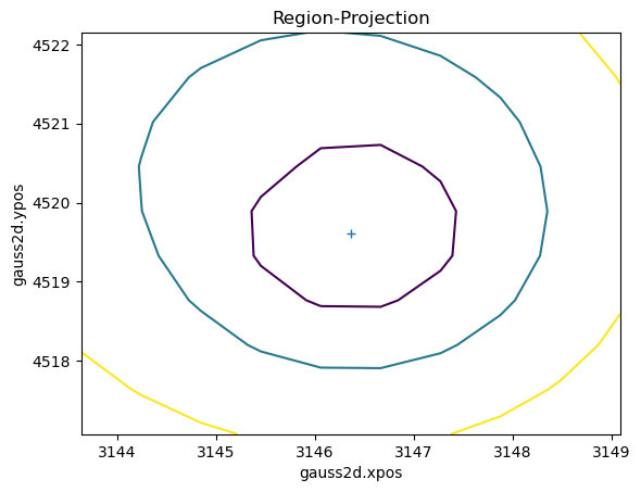
[35]:
ui.get_reg_proj()
[35]: