Sherpa Quick Start
This tutorial shows some basic Sherpa features. More information on Sherpa can be found in the Sherpa documentation.
Workflow:
create synthetic data: a parabola with noise and error bars
load data in Sherpa
plot data using matplotlib
set, inspect, edit a model to fit the data
fit the data
compute the confidence intervals for the parameters
explore the parameter space
First of all, let’s activate the inline matplotlib mode. Sherpa seamlessly uses matplotlib to provide immediate visual feedback to the user. Support for matplotlib in Sherpa requires the matplotlib package to be installed.
[1]:
%matplotlib inline
Now, let’s create a simple synthetic dataset, using numpy: a parabola between x=-5 and x=5, with some randomly generated noise (the form for y is chosen to match the model selected in step 6 below to fit the data, and the random seed used by NumPy is set to make this notebook repeatable):
[2]:
import numpy as np
np.random.seed(824842)

x = np.arange(-5, 5.1)

c0_true = 23.2
c1_true = 0
c2_true = 1

y = c2_true * x*x + c1_true * x + c0_true + np.random.normal(size=x.size)
e = np.ones(x.size)
Let’s import Sherpa:
[3]:
from sherpa.astro import ui
WARNING: imaging routines will not be available,
failed to import sherpa.image.ds9_backend due to
'RuntimeErr: DS9Win unusable: Could not find ds9 on your PATH'
Depending on how you installed Sherpa, certain special features may be enabled or disabled. Sherpa prints some warning messages when it cannot find some of its modules, as shown above. These warnings are benign. You can refer to the Sherpa documentation to find out what additional features you can enable in Sherpa and how to enable them.
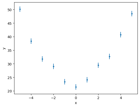
Let’s load and plot the data we just created. Notice we are assigning the ID mydata to the dataset we are loading. We will use this ID to refer to the same dataset in the rest of the tutorial. Sherpa can deal with multiple datasets, fit them simultaneously with the same model, and even link parameters between models. Sherpa can read ASCII table and FITS files (provided the astropy package is installed).
[4]:
ui.load_arrays("mydata", x, y, e)
ui.plot_data("mydata")
The data can be retrieved with the get_data routine:
[5]:
d = ui.get_data("mydata")
print(d)
name      =
x         = Float64[11]
y         = Float64[11]
staterror = Float64[11]
syserror  = None
The object - in this case a Data1D object - has support for Jupyter notebooks and will display a summary of the data (in this case a plot, but other objects will display differently, as we will see below):
[6]:
d
[6]:
Data1D Plot
We can set the model we want to fit to the data using the set_model call. There are different ways to instantiate the models: in this case, we just use the string polynom1d to refer to a 1D polynomial. The name of the model will be poly, and will be accessible as a Python variable. One can use more object oriented patterns to access and instantiate built-in models. Also, new models can be added by the user as Python functions or from tabular data.
[7]:
ui.set_model("mydata", "polynom1d.poly")
Several Sherpa commands can be used to inspect the model. In this case we just use a simple print to get a summary of the model and its components.
[8]:
print(poly)
polynom1d.poly
   Param        Type          Value          Min          Max      Units
   -----        ----          -----          ---          ---      -----
   poly.c0      thawed            1 -3.40282e+38  3.40282e+38
   poly.c1      frozen            0 -3.40282e+38  3.40282e+38
   poly.c2      frozen            0 -3.40282e+38  3.40282e+38
   poly.c3      frozen            0 -3.40282e+38  3.40282e+38
   poly.c4      frozen            0 -3.40282e+38  3.40282e+38
   poly.c5      frozen            0 -3.40282e+38  3.40282e+38
   poly.c6      frozen            0 -3.40282e+38  3.40282e+38
   poly.c7      frozen            0 -3.40282e+38  3.40282e+38
   poly.c8      frozen            0 -3.40282e+38  3.40282e+38
   poly.offset  frozen            0 -3.40282e+38  3.40282e+38
We can also display it directly in a Jupyter notebook:
[9]:
poly
[9]:
Model
| Component | Parameter | Thawed | Value | Min | Max | Units |
|---|---|---|---|---|---|---|
| polynom1d.poly | c0 | 1.0 | -MAX | MAX | ||
| c1 | 0.0 | -MAX | MAX | |||
| c2 | 0.0 | -MAX | MAX | |||
| c3 | 0.0 | -MAX | MAX | |||
| c4 | 0.0 | -MAX | MAX | |||
| c5 | 0.0 | -MAX | MAX | |||
| c6 | 0.0 | -MAX | MAX | |||
| c7 | 0.0 | -MAX | MAX | |||
| c8 | 0.0 | -MAX | MAX | |||
| offset | 0.0 | -MAX | MAX |
By default, only the first component (the intercept) is thawed, i.e. is free to vary in the fit. This corresponds to a constant function. In order to fit a parabola, we need to thaw the coefficients of the first two orders in the polynomial, as shown below.
[10]:
ui.thaw(poly.c1, poly.c2)
We are going to fit the dataset using the default settings. However, Sherpa has a number of optimization algorithms, each configurable by the user, and a number of statistics that can be used to take into account the error and other characteristics of data being fitted.
[11]:
ui.fit("mydata")
Dataset               = mydata
Method                = levmar
Statistic             = chi2
Initial fit statistic = 12642.8
Final fit statistic   = 15.643 at function evaluation 8
Data points           = 11
Degrees of freedom    = 8
Probability [Q-value] = 0.0477837
Reduced statistic     = 1.95538
Change in statistic   = 12627.2
   poly.c0        23.1367      +/- 0.455477
   poly.c1        0.0537585    +/- 0.0953463
   poly.c2        1.04602      +/- 0.0341394
Notice that Sherpa used a Levenberg-Marquadt minimization strategy (levmar), and the \(\chi^2\) error function (chi2). These options can be changed with the set_method and set_stat functions. Note that when using the levmar optimiser the fit results include approximate error estimates, but you should use the conf routine (shown below) to get accurate error estimates.
The best fit values of the parameters are close to the ones defined when we generated the dataset:
Parameter |
true value |
best-fit value |
|---|---|---|
\(c_0\) |
23.2 |
23.1367 |
\(c_1\) |
0 |
0.0538 |
\(c_2\) |
1 |
1.0460 |
The get_fit_results function will return the information on the last fit:
[12]:
fitres = ui.get_fit_results()
print(fitres)
datasets       = ('mydata',)
itermethodname = none
methodname     = levmar
statname       = chi2
succeeded      = True
parnames       = ('poly.c0', 'poly.c1', 'poly.c2')
parvals        = (23.136688550821013, 0.05375853511753547, 1.046015029290237)
statval        = 15.6430444797243
istatval       = 12642.832375778722
dstatval       = 12627.189331298998
numpoints      = 11
dof            = 8
qval           = 0.04778369987400388
rstat          = 1.9553805599655374
message        = successful termination
nfev           = 8
Perhaps unsurprisingly by now, it too can be displayed automatically in a Jupyter notebook:
[13]:
fitres
[13]:
Fit parameters
| Parameter | Best-fit value | Approximate error |
|---|---|---|
| poly.c0 | 23.1367 | ± 0.455477 |
| poly.c1 | 0.0537585 | ± 0.0953463 |
| poly.c2 | 1.04602 | ± 0.0341394 |
Summary (11)
The model object has also been updated by the fit:
[14]:
poly
[14]:
Model
| Component | Parameter | Thawed | Value | Min | Max | Units |
|---|---|---|---|---|---|---|
| polynom1d.poly | c0 | 23.136688550821013 | -MAX | MAX | ||
| c1 | 0.05375853511753547 | -MAX | MAX | |||
| c2 | 1.046015029290237 | -MAX | MAX | |||
| c3 | 0.0 | -MAX | MAX | |||
| c4 | 0.0 | -MAX | MAX | |||
| c5 | 0.0 | -MAX | MAX | |||
| c6 | 0.0 | -MAX | MAX | |||
| c7 | 0.0 | -MAX | MAX | |||
| c8 | 0.0 | -MAX | MAX | |||
| offset | 0.0 | -MAX | MAX |
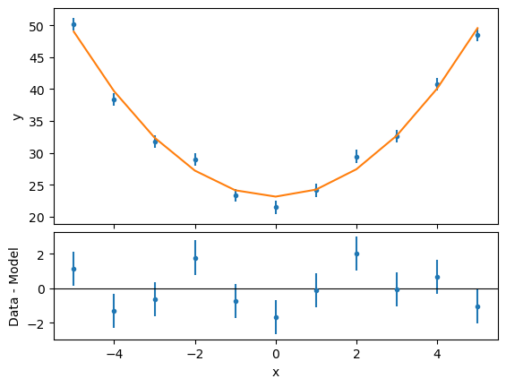
In order to get immediate feedback of the fit results, we can plot the fit and the residuals. Again, Sherpa facilitates the creation of the plots, but users can harvest the power of matplotlib directly if they want to.
[15]:
ui.plot_fit_resid("mydata")
We can now compute the confidence intervals for the free parameters in the fit:
[16]:
ui.conf("mydata")
poly.c0 lower bound:    -0.455477
poly.c1 lower bound:    -0.0953463
poly.c0 upper bound:    0.455477
poly.c1 upper bound:    0.0953463
poly.c2 lower bound:    -0.0341394
poly.c2 upper bound:    0.0341394
Dataset               = mydata
Confidence Method     = confidence
Iterative Fit Method  = None
Fitting Method        = levmar
Statistic             = chi2gehrels
confidence 1-sigma (68.2689%) bounds:
   Param            Best-Fit  Lower Bound  Upper Bound
   -----            --------  -----------  -----------
   poly.c0           23.1367    -0.455477     0.455477
   poly.c1         0.0537585   -0.0953463    0.0953463
   poly.c2           1.04602   -0.0341394    0.0341394
[17]:
conf = ui.get_conf_results()
print(conf)
datasets    = ('mydata',)
methodname  = confidence
iterfitname = none
fitname     = levmar
statname    = chi2gehrels
sigma       = 1
percent     = 68.26894921370858
parnames    = ('poly.c0', 'poly.c1', 'poly.c2')
parvals     = (23.136688550821013, 0.05375853511753547, 1.046015029290237)
parmins     = (-0.4554769011263424, -0.09534625892453424, -0.03413943709996614)
parmaxes    = (0.4554769011263424, 0.09534625892453424, 0.03413943709996614)
nfits       = 6
or, if you want a fancy display, you can get the Jupter notebook to display it:
[18]:
conf
[18]:
confidence 1σ (68.2689%) bounds
| Parameter | Best-fit value | Lower Bound | Upper Bound |
|---|---|---|---|
| poly.c0 | 23.1367 | -0.455477 | 0.455477 |
| poly.c1 | 0.0537585 | -0.0953463 | 0.0953463 |
| poly.c2 | 1.04602 | -0.0341394 | 0.0341394 |
Summary (3)
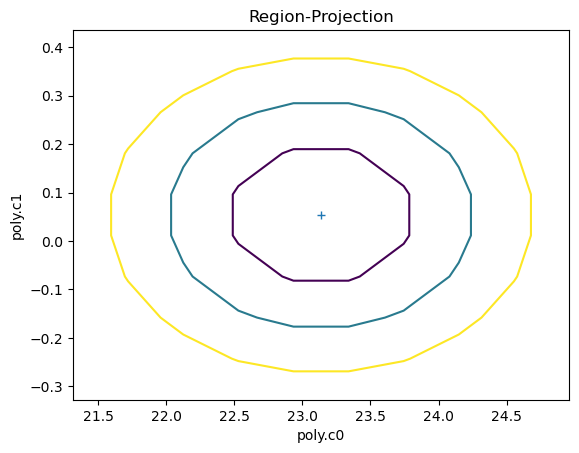
Sherpa allows to inspect the parameter space. In the cell below we ask sherpa to show us the projection of the confidence regions for the c0 and c1 parameters. The contours are configurable by the user: by default they show the confidence curves at 1, 2, and 3 \(\sigma\)
[19]:
ui.reg_proj(poly.c0, poly.c1)
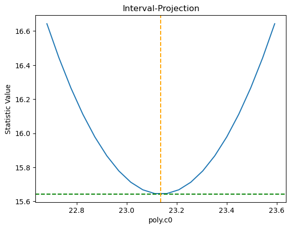
We can also directlty inspect the parameter space. For instance, in the plot below Sherpa displays the Interval Projection of the c0 parameter, i.e. a plot of the error for each value of the parameter, around the minimum found by the optimization method during the fit.
[20]:
ui.int_proj(poly.c0)