What data is to be fit?
The Sherpa Data class is used to
carry around the data to be fit: this includes the independent
axis (or axes), the dependent axis (the data), and any
necessary metadata. Although the design of Sherpa supports
multiple-dimensional data sets, the current classes only
support one- and two-dimensional data sets.
The following modules are assumed to have been imported:
>>> import numpy as np
>>> import matplotlib.pyplot as plt
>>> from sherpa.stats import LeastSq
>>> from sherpa.optmethods import LevMar
>>> from sherpa import data
Names
The first argument to any of the Data classes is the name
of the data set. This is used for display purposes only,
and can be useful to identify which data set is in use.
It is stored in the name attribute of the object, and
can be changed at any time.
The independent axis
The independent axis - or axes - of a data set define the
grid over which the model is to be evaluated. It is referred
to as x, x0, x1, … depending on the dimensionality
of the data (for
binned datasets there are lo
and hi variants).
Although dense multi-dimensional data sets can be stored as arrays with dimensionality greater than one, the internal representation used by Sherpa is often a flattened - i.e. one-dimensional - version.
The sherpa.astro.data.DataPHA class can be thought of
as being either unbinned or binned, depending on the units
(channels or energy/wavelength), and this is discussed in the
PHA example page.
The dependent axis
This refers to the data being fit, and is referred to as y.
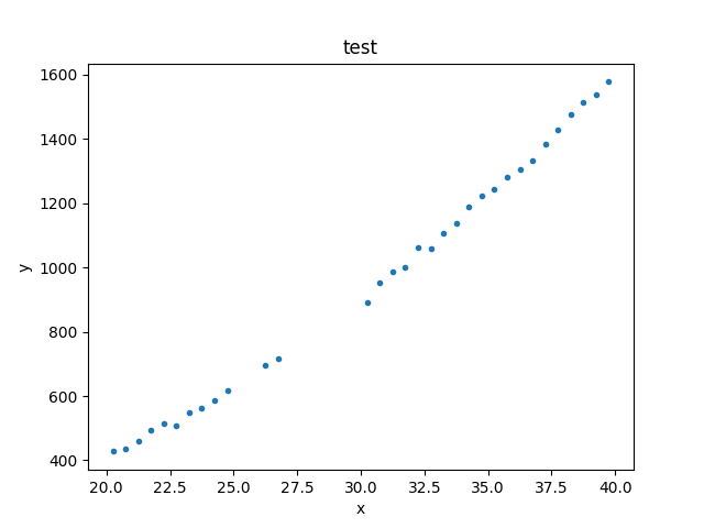
Unbinned data
Unbinned data sets - defined by classes which do not end in
the name Int - represent point values; that is, the the data
value is the value at the coordinates given by the independent
axis.
Examples of unbinned data classes are
Data1D and Data2D.
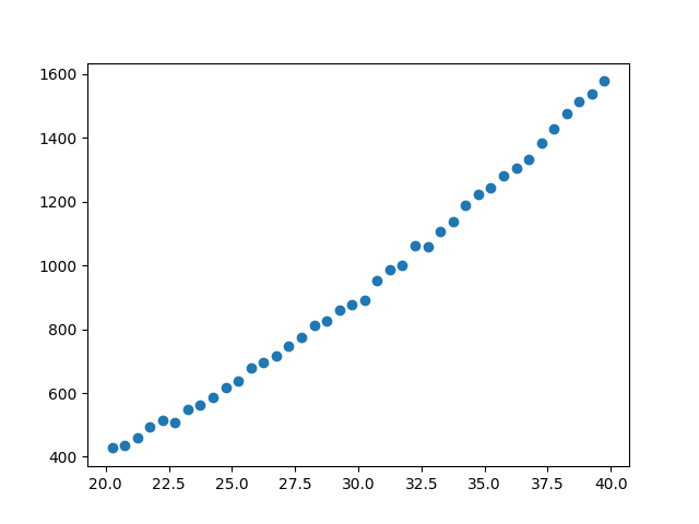
>>> np.random.seed(0)
>>> x = np.arange(20.25, 40, 0.5)
>>> y = x**2 + np.random.normal(0, 10, size=x.size)
>>> d1 = data.Data1D('test', x, y)
>>> print(d1)
name      = test
x         = Float64[40]
y         = Float64[40]
staterror = None
syserror  = None
>>> print(d1.x)
[20.25 20.75 21.25 21.75 22.25 22.75 23.25 23.75 24.25 24.75 25.25 25.75
 26.25 26.75 27.25 27.75 28.25 28.75 29.25 29.75 30.25 30.75 31.25 31.75
 32.25 32.75 33.25 33.75 34.25 34.75 35.25 35.75 36.25 36.75 37.25 37.75
 38.25 38.75 39.25 39.75]
>>> print(d1.y)
[ 427.70302346  434.56407208  461.34987984  495.47143199  513.7380799
  507.7897212   550.06338418  562.54892792  587.03031148  616.66848502
  639.00293571  677.60523507  696.67287725  716.77925016  747.00113233
  773.39924327  813.00329073  824.51091736  858.69317702  876.52154261
  889.53260184  952.09868595  985.20686199 1000.6408498  1062.76004624
 1058.01884325 1106.02008517 1137.1906615  1188.39029214 1222.2560877
 1244.11197426 1281.8441252  1305.18464252 1330.75453532 1384.08337851
 1426.62598969 1475.36540681 1513.58629849 1536.68923183 1577.03947249]
>>> plt.plot(d.x, d.y, 'o')
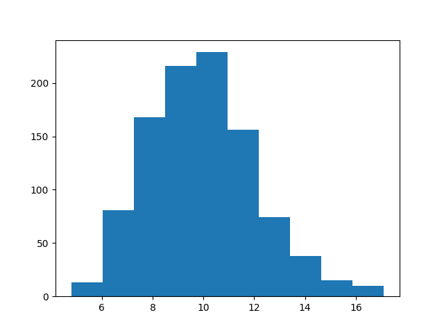
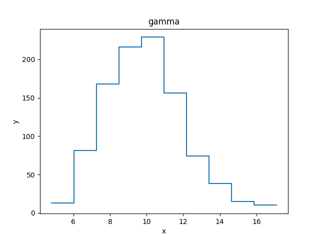
Binned data
Binned data sets represent values that are defined over a range,
such as a histogram.
The integrated model classes end in Int: examples are
Data1DInt
and Data2DInt.
It can be a useful optimisation to treat a binned data set as an unbinned one, since it avoids having to estimate the integral of the model over each bin. It depends in part on how the bin size compares to the scale over which the model changes.
>>> z = np.random.gamma(20, scale=0.5, size=1000)
>>> (y, edges) = np.histogram(z)
>>> d2 = data.Data1DInt('gamma', edges[:-1], edges[1:], y)
>>> print(d2)
name      = gamma
xlo       = Float64[10]
xhi       = Float64[10]
y         = Int64[10]
staterror = None
syserror  = None
>>> plt.clf()
>>> plt.bar(d2.xlo, d2.y, d2.xhi - d2.xlo, align='edge')
Errors
There is support for both statistical and systematic
errors by either using the staterror and syserror
parameters when creating the data object, or by changing the
staterror and
syserror attributes of the object.
Filtering data
Sherpa supports filtering data sets; that is, temporarily removing parts of the data (perhaps because there are problems, or to help restrict parameter values). There are routines to filter the data and to find out what bins have been selected.
Note
Sherpa has limited support for Numpy masked arrays. This is only applied to the dependent axis; that is, masked values are ignored when found on any other field, including the independent axes, error values, and the mask attribute.
On reading in a Numpy masked array, the mask values will be
converted, since in Sherpa a mask value of True means the value
is included and False the value is excluded.
The ignore() and
notice() methods are used to
define the ranges to exclude or include.
The mask attribute indicates
whether a filter has been applied: if it returns True then
no filter is set, False when all data has been filtered out,
otherwise it is a bool array
where False values indicate those elements that are to be
ignored.
Note that the Sherpa definition is opposite of the convention in numpy, where True indicates
a masked value to be ignored, while Sherpa uses False for this purpose.
For example, the following
hides those values where the independent axis values are between
21.2 and 22.8:
>>> d1.ignore(21.2, 22.8)
>>> d1.x[np.invert(d1.mask)]
array([21.25, 21.75, 22.25, 22.75])
Note
The meaning of the range selected by the notice and ignore calls
depends on the data class: sherpa.data.Data1DInt and
sherpa.astro.data.DataPHA classes can treat the
upper limit differently (it can be inclusive or exclusive)
and 2D datasets such as sherpa.data.Data2D can
use filters that use both axes.
The get_filter() method will report a
string representation of the existing filter, so here showing that
the bins between 21.2 and 22.8 have been ignored:
>>> print(d1.get_fiter())
20.2500:20.7500,23.2500:39.7500
Note
The filter does not record the requested changes - that is here
the 21.2 to 22.8 arguments to ignore() -
but instead reflects the selected bins in the data set.
After this, a fit to the data will ignore these values, as shown
below, where the number of degrees of freedom of the first fit,
which uses the filtered data, is three less than the fit to the
full data set (the call to
notice() removes the filter since
no arguments were given):
>>> from sherpa.models import Polynom1D
>>> from sherpa.fit import Fit
>>> mdl = Polynom1D()
>>> mdl.c2.thaw()
>>> fit = Fit(d1, mdl, stat=LeastSq(), method=LevMar())
>>> res1 = fit.fit()

>>> d1.notice()
>>> res2 = fit.fit()

>>> print(f"Degrees of freedom: {res1.dof} vs {res2.dof}")
Degrees of freedom: 34 vs 38
Resetting the filter
The notice() method can be used to
reset the filter - that is, remove all filters - by calling with no
arguments (or, equivalently, with two None arguments). Similarly
the ignore() method called with no
arguments will remove all points.
The first filter call
When a data set is created no filter is applied, which is treated
as a special case (this also holds if the
filters have been reset).
The first call to notice()
will restrict the data to just the requested range, and subsequent
calls will add the new data. So with no filter we see the whole data
range:
>>> d1.notice()
>>> print(d1.get_fiter(format='%.2f'))
20.25:39.75
The first notice() call restricts to just
this range:
>>> d1.notice(25, 27)
>>> print(d1.get_fiter(format='%.1f'))
25.25:26.75
Subsequent notice() calls add to the selected
range:
>>> d1.notice(30, 35)
>>> print(d1.get_fiter(format='%.1f'))
25.25:26.75,30.25:34.75
The edges of a filter
Mathematically the two sets of commands below should select the same
range, but it can behave slightly different for values at the edge
of the filter (or within the edge bins for Data1DInt
and DataPHA objects):
>>> d1.notice(25, 35)
>>> d1.ignore(29, 31)
>>> d1.notice(25, 29)
>>> d1.notice(31, 35)
Accessing filtered data
Although the mask attribute can be used
to manually filter the data, many data accessors accept a filter
argument which, if set, will filter the requested data. When a filter
is applied, get_x() and
get_y() will default to returning all the
data but if the filter argument is set then the current filter
will be applied:
>>> d1.notice()
>>> d1.notice(21.1, 23.5)
>>> d1.get_x()
[20.25 20.75 21.25 21.75 22.25 22.75 23.25 23.75 24.25 24.75 25.25 25.75
 26.25 26.75 27.25 27.75 28.25 28.75 29.25 29.75 30.25 30.75 31.25 31.75
 32.25 32.75 33.25 33.75 34.25 34.75 35.25 35.75 36.25 36.75 37.25 37.75
 38.25 38.75 39.25 39.75]
>>> d1.get_y()
[ 427.70302346  434.56407208  461.34987984  495.47143199  513.7380799
  507.7897212   550.06338418  562.54892792  587.03031148  616.66848502
  639.00293571  677.60523507  696.67287725  716.77925016  747.00113233
  773.39924327  813.00329073  824.51091736  858.69317702  876.52154261
  889.53260184  952.09868595  985.20686199 1000.6408498  1062.76004624
 1058.01884325 1106.02008517 1137.1906615  1188.39029214 1222.2560877
 1244.11197426 1281.8441252  1305.18464252 1330.75453532 1384.08337851
 1426.62598969 1475.36540681 1513.58629849 1536.68923183 1577.03947249]
>>> d1.get_x(filter=True)
[21.25 21.75 22.25 22.75 23.25]
>>> d1.get_y(filter=True)
[461.34987984 495.47143199 513.7380799  507.7897212  550.06338418]
Enhanced filtering
Certain data classes - in particular sherpa.astro.data.DataIMG
and sherpa.astro.data.DataPHA - extend and enhance the
filtering capabilities to:
Visualizing a data set
The data objects contain several methods which can be used to
visualize the data, but do not provide any direct plotting
or display capabilities. There are low-level routines which
provide access to the data - these include the
to_plot() and
to_contour() methods - but the
preferred approach is to use the classes defined in the
sherpa.plot module, which are described in the
visualization section:
>>> from sherpa.plot import DataHistogramPlot
>>> pdata = DataHistogramPlot()
>>> pdata.prepare(d2)
>>> pdata.plot()
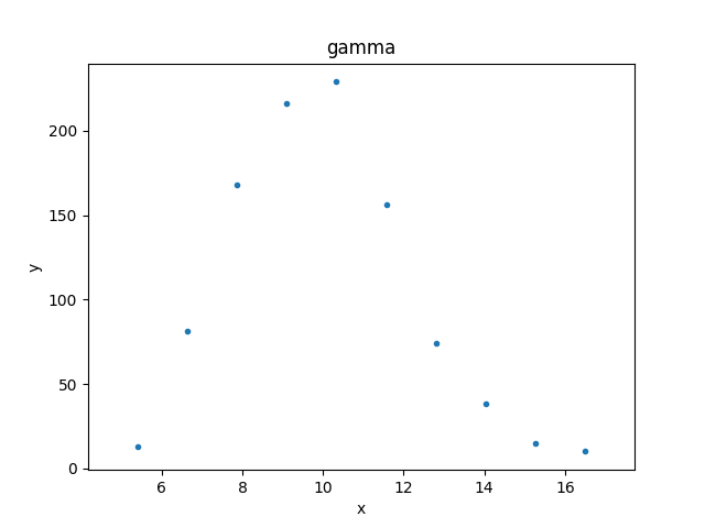
Although the data represented by d2 is
a histogram, the values are displayed at the center of the bin.
Plot preferences can be changed in the plot call:
>>> pdata.plot(linestyle='solid', marker='')
Note
The supported options depend on the plot backend (although at present only matplotlib is supported).
The plot objects automatically handle any filters applied to the data, as shown below.
>>> from sherpa.plot import DataPlot
>>> pdata = DataPlot()
>>> d1.notice()
>>> d1.ignore(25, 30)
>>> d1.notice(26, 27)
>>> pdata.prepare(d1)
>>> pdata.plot()
Note
The plot object stores the data given in the
prepare() call,
so that changes to the underlying objects will not be reflected
in future calls to
plot()
unless a new call to
prepare() is made.
>>> d1.notice()
At this point, a call to pdata.plot() would re-create the previous
plot, even though the filter has been removed from the underlying
data object.
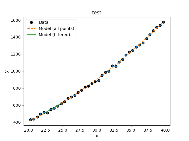
Evaluating a model
The eval_model() and
eval_model_to_fit()
methods can be used
to evaluate a model on the grid defined by the data set. The
first version uses the full grid, whereas the second respects
any filtering applied to the data.
>>> d1.notice(22, 25)
>>> y1 = d1.eval_model(mdl)
>>> y2 = d1.eval_model_to_fit(mdl)
>>> x2 = d1.x[d1.mask]
>>> plt.plot(d1.x, d1.y, 'ko', label='Data')
>>> plt.plot(d1.x, y1, '--', label='Model (all points)')
>>> plt.plot(x2, y2, linewidth=2, label='Model (filtered)')
>>> plt.legend(loc=2)