Writing your own model
A model class can be created to fit any function, or interface with external code.
Overview
A single model is defined by the parameters of the model - stored
as sherpa.models.parameter.Parameter instances - and the function that
takes the parameter values along with an array of grid values to calculate
values of the model. This is packaged together in a class for each model,
and instances of this class can then be used to fit data.
Sherpa provides several base classes in sherpa.models.model; the most
commonly used ones are:
ArithmeticModelis the main base class for deriving user models since it supports combining models (e.g. by addition or multiplication) and a cache to reduce evaluation time at the expense of memory use.ArithmeticConstantModelandmodelArithmeticFunctionModelare less general thanArithmeticModeland can be used to represent a constant value or a function.RegriddableModel1DandRegriddableModel2Dwhich build onArithmeticModelto allow a model to be evaluated on a separate grid and then re-binned or interpolated onto the requested grid.
To define a new model, a new class inherits from one of these base classes and
implements an __init__ method that defines the model parameters
and a calc method that, given the parameter values and the coordinates
at which the model is to be evaluated, returns the model values.
Calculating the model values
Many Sherpa models are set up to work with both integrated and non-integrated data,
some might even work with data of different dimensionality. Because of that, the input
to the calc method can take several forms:
For
Data1Ddata, the input iscalc(pars, x, **kwargs)For
Data1DIntdata, the input iscalc(pars, xlo, xhi, **kwargs), wherexloandxhiare the lower and upper bounds of the bins in the independent coordinate.For
Data2Ddata, the input iscalc(pars, x0, x1, **kwargs).x0andx1are flattened arrays for the two independent coordinates, so they are one-dimensional.For
Data2DIntdata, the input iscalc(pars, x0lo, x1lo, x0hi, x1hi, **kwargs). Here,x0loandx0hiare the lower and upper bounds of the bins in the first coordinate of the independent variable, andx1loandx1hiare the lower and upper bounds of the bins in the second coordinate.For
DataPHAdata, the input iscalc(pars, xlo, xhi, **kwargs), where x could be given in either energy or wavelength units, depending on the setting ofset_analysis.
Sherpa provides other data classes and users can implement their own data classes, that might follow different conventions, but the cases listed above cover the typical use of Sherpa.
In all cases, **kwargs are keywords that the model might accept (this feature is not used
by most Sherpa models) and pars is a list of parameter values, in the same order as they are
listed in the model instances:
>>> from sherpa.models.basic import Gauss1D
>>> mdl = Gauss1D(name='mygauss')
>>> print([p.fullname for p in mdl.pars])
['mygauss.fwhm', 'mygauss.pos', 'mygauss.ampl']
Often, in Sherpa, we want models to work with both integrated and non-integrated datasets, and thus
calc is defined to accept a flexible number of arguments. In the most general form,
you can use def calc(self, pars, *args, **kwargs) and the code in calc can branch
depending on how long *args. For a 1D model, you can also say
def calc(self, pars, x, xhi=None, **kwargs) and then xhi will be None for non-integrated
data; the same works similarly for 2D data.
Here is an example for a 1D model:
>>> from sherpa.models import model
>>> class LinearModel(model.RegriddableModel1D):
...     def __init__(self, name='linemodel'):
...         self.slope = model.Parameter(name, 'slope', 1, min=-10, hard_min=-1e20, max=10, hard_max=1e20)
...         super().__init__(name, (self.slope, ))
...
...     def calc(self, pars, *args, **kwargs):
...         if len(args) == 1:
...             return args[0] * pars[0]
...         elif len(args) == 2:
...             xlo, xhi = args
...             return (xlo + xhi) / 2 * pars[0]
...         else:
...             raise ValueError('This model only works in 1 dimension')
For a linear model, the integrated value over the bin is just the linear model evaluated in the middle of the bin, but in general, the implementation can be more complex.
We can now evaluate this model for points or for bins:
>>> import numpy as np
>>> linear = LinearModel()
>>> linear.calc([2], np.array([1.3, 3.4]))
array([2.6, 6.8])
>>> linear.calc([2.], np.array([0, 2, 3]), np.array([2, 3, 5]))
array([2., 5., 8.])
In the examples below, we will set up full data classes and fits and not just pass
the numbers directly into the calc method.
Dimensionality of the data and the model
Most models only work for either 1D or 2D data, or some other specific dimension and,
for example, adding a 1D model expression to a 2D model does not make sense and won’t work. Sherpa
performs some checks on that using the ndim attribute of a model.
In the example code above, we do not need to set
ndim, because it is inherited from
sherpa.models.model.RegriddableModel1D:
>>> linear.ndim
1
However, if a new user model inherits from one of the more general classes such as
ArithmeticModel, then the ndim
attribute should be set.
A one-dimensional model
An example is a function similar to the AstroPy trapezoidal model, which has four parameters: the amplitude of the central region, the center and width of this region, and the slope. The following model class, which was not written for efficiency or robustness, implements this interface:
>>> def _trap1d(pars, x):
...     """Evaluate the Trapezoid.
...
...     Parameters
...     ----------
...     pars: sequence of 4 numbers
...         The order is amplitude, center, width, and slope.
...         These numbers are assumed to be valid (e.g. width
...         is 0 or greater).
...     x: sequence of numbers
...         The grid on which to evaluate the model. It is expected
...         to be a floating-point type.
...
...     Returns
...     -------
...     y: sequence of numbers
...         The model evaluated on the input grid.
...     """
...
...     (amplitude, center, width, slope) = pars
...
...     # There are five segments:
...     #    xlo = center - width/2
...     #    xhi = center + width/2
...     #    x0  = xlo - amplitude/slope
...     #    x1  = xhi + amplitude/slope
...     #
...     #    flat   xlo <= x < xhi
...     #    slope  x0 <= x < xlo
...     #           xhi <= x < x1
...     #    zero   x < x0
...     #           x >= x1
...     #
...     hwidth = width / 2.0
...     dx = amplitude / slope
...     xlo = center - hwidth
...     xhi = center + hwidth
...     x0 = xlo - dx
...     x1 = xhi + dx
...
...     out = np.zeros(x.size)
...     out[(x >= xlo) & (x < xhi)] = amplitude
...
...     idx = np.where((x >= x0) & (x < xlo))
...     out[idx] = slope * x[idx] - slope * x0
...
...     idx = np.where((x >= xhi) & (x < x1))
...     out[idx] = - slope * x[idx] + slope * x1
...
...     return out
>>> from sherpa.models import model
>>> class Trap1D(model.RegriddableModel1D):
...     """A one-dimensional trapezoid.
...
...     The model parameters are:
...
...     ampl
...        The amplitude of the central (flat) segment (zero or greater).
...     center
...        The center of the central segment.
...     width
...        The width of the central segment (zero or greater).
...     slope
...         The gradient of the slopes (zero or greater).
...     """
...
...     def __init__(self, name='trap1d'):
...         self.ampl = model.Parameter(name, 'ampl', 1, min=0, hard_min=0)
...         self.center = model.Parameter(name, 'center', 1)
...         self.width = model.Parameter(name, 'width', 1, min=0, hard_min=0)
...         self.slope = model.Parameter(name, 'slope', 1, min=0, hard_min=0)
...         super().__init__(name,
...                          (self.ampl, self.center, self.width, self.slope))
...
...     def calc(self, pars, x, *args, **kwargs):
...         """Evaluate the model"""
...
...         # If given an integrated data set, use the center of the bin
...         if len(args) == 1:
...             x = (x + args[0]) / 2
...
...         return _trap1d(pars, x)
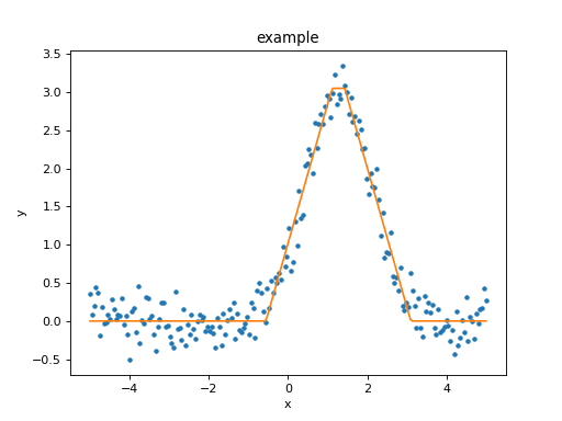
This can be used in the same manner as the
Gauss1D model
in the quick guide to Sherpa.
First, create the data to fit:
>>> import numpy as np
>>> import matplotlib.pyplot as plt
>>> np.random.seed(0)
>>> x = np.linspace(-5., 5., 200)
>>> ampl_true = 3
>>> pos_true = 1.3
>>> sigma_true = 0.8
>>> err_true = 0.2
>>> y = ampl_true * np.exp(-0.5 * (x - pos_true)**2 / sigma_true**2)
>>> y += np.random.normal(0., err_true, x.shape)
Now create a Sherpa data object and set up the user model:
>>> from sherpa.data import Data1D
>>> d = Data1D('example', x, y)
>>> t = Trap1D()
>>> print(t)
trap1d
   Param        Type          Value          Min          Max      Units
   -----        ----          -----          ---          ---      -----
   trap1d.ampl  thawed            1            0  3.40282e+38
   trap1d.center thawed            1 -3.40282e+38  3.40282e+38
   trap1d.width thawed            1            0  3.40282e+38
   trap1d.slope thawed            1            0  3.40282e+38
Finally, perform the fit:
>>> from sherpa.fit import Fit
>>> from sherpa.stats import LeastSq
>>> from sherpa.optmethods import LevMar
>>> tfit = Fit(d, t, stat=LeastSq(), method=LevMar())
>>> tres = tfit.fit()
>>> if not tres.succeeded: print(tres.message)
Rather than use a ModelPlot object,
the overplot argument can be set to allow multiple values
in the same plot:
>>> from sherpa import plot
>>> dplot = plot.DataPlot()
>>> dplot.prepare(d)
>>> dplot.plot()
>>> mplot = plot.ModelPlot()
>>> mplot.prepare(d, t)
>>> mplot.plot(overplot=True)
A two-dimensional model
The two-dimensional case is similar to the one-dimensional case,
with the major difference being the number of independent axes to
deal with. In the following example the model is assumed to only be
applied to non-integrated data sets, as it simplifies the implementation
of the calc method.
It also shows one way of embedding models from a different system, in this case the two-dimemensional polynomial model from the AstroPy package:
>>> from astropy.modeling.polynomial import Polynomial2D
>>> class WrapPoly2D(model.RegriddableModel2D):
...     """A two-dimensional polynomial from AstroPy, restricted to degree=2.
...
...     The model parameters (with the same meaning as the underlying
...     AstroPy model) are:
...
...     c0_0
...     c1_0
...     c2_0
...     c0_1
...     c0_2
...     c1_1
...     """
...     def __init__(self, name='wrappoly2d'):
...         self._actual = Polynomial2D(degree=2)
...         self.c0_0 = model.Parameter(name, 'c0_0', 0)
...         self.c1_0 = model.Parameter(name, 'c1_0', 0)
...         self.c2_0 = model.Parameter(name, 'c2_0', 0)
...         self.c0_1 = model.Parameter(name, 'c0_1', 0)
...         self.c0_2 = model.Parameter(name, 'c0_2', 0)
...         self.c1_1 = model.Parameter(name, 'c1_1', 0)
...
...         super().__init__(name,
...                          (self.c0_0, self.c1_0, self.c2_0,
...                           self.c0_1, self.c0_2, self.c1_1))
...
...     def calc(self, pars, x0, x1, *args, **kwargs):
...         """Evaluate the model"""
...
...         # This does not support 2D integrated data sets
...         mdl = self._actual
...         for n in ['c0_0', 'c1_0', 'c2_0', 'c0_1', 'c0_2', 'c1_1']:
...             pval = getattr(self, n).val
...             getattr(mdl, n).value = pval
...
...         return mdl(x0, x1)
Repeating the 2D fit by first setting up the data to fit:
>>> np.random.seed(0)
>>> y2, x2 = np.mgrid[:128, :128]
>>> z = 2. * x2 ** 2 - 0.5 * y2 ** 2 + 1.5 * x2 * y2 - 1.
>>> z += np.random.normal(0., 0.1, z.shape) * 50000.
Put this data into a Sherpa data object:
>>> from sherpa.data import Data2D
>>> x0axis = x2.ravel()
>>> x1axis = y2.ravel()
>>> d2 = Data2D('img', x0axis, x1axis, z.ravel(), shape=(128,128))
Create an instance of the user model:
>>> wp2 = WrapPoly2D('wp2')
>>> wp2.c1_0.frozen = True
>>> wp2.c0_1.frozen = True
Finally, perform the fit:
>>> f2 = Fit(d2, wp2, stat=LeastSq(), method=LevMar())
>>> res2 = f2.fit()
>>> if not res2.succeeded: print(res2.message)
>>> print(res2)
datasets       = None
itermethodname = none
methodname     = levmar
statname       = leastsq
succeeded      = True
parnames       = ('wp2.c0_0', 'wp2.c2_0', 'wp2.c0_2', 'wp2.c1_1')
parvals        = (-80.289475553599914, 1.9894112623565667, -0.4817452191363118, 1.5022711710873158)
statval        = 400658883390.6685
istatval       = 6571934382318.328
dstatval       = 6.17127549893e+12
numpoints      = 16384
dof            = 16380
qval           = None
rstat          = None
message        = successful termination
nfev           = 80
>>> print(wp2)
wp2
   Param        Type          Value          Min          Max      Units
   -----        ----          -----          ---          ---      -----
   wp2.c0_0     thawed     -80.2895 -3.40282e+38  3.40282e+38
   wp2.c1_0     frozen            0 -3.40282e+38  3.40282e+38
   wp2.c2_0     thawed      1.98941 -3.40282e+38  3.40282e+38
   wp2.c0_1     frozen            0 -3.40282e+38  3.40282e+38
   wp2.c0_2     thawed    -0.481745 -3.40282e+38  3.40282e+38
   wp2.c1_1     thawed      1.50227 -3.40282e+38  3.40282e+38