Simulating data
A simple case
Simulating a data set normally involves:
evaluate the model
add in noise
This may need to be repeated several times for complex models, such as when different components have different noise models or the noise needs to be added before evaluation by a component.
The model evaluation would be performed using the techniques
described in this section, and then the noise term can be
handled with sherpa.utils.poisson_noise() or routines from
NumPy or SciPy
to evaluate noise.
>>> import numpy as np
>>> from sherpa.models.basic import Polynom1D
>>> x = np.arange(10, 100, 12)
>>> mdl = Polynom1D('mdl')
>>> mdl.offset = 35
>>> mdl.c1 = 0.5
>>> mdl.c2 = 0.12
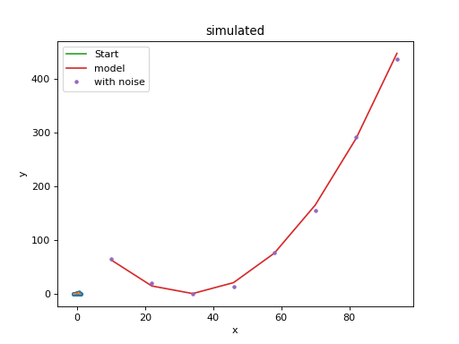
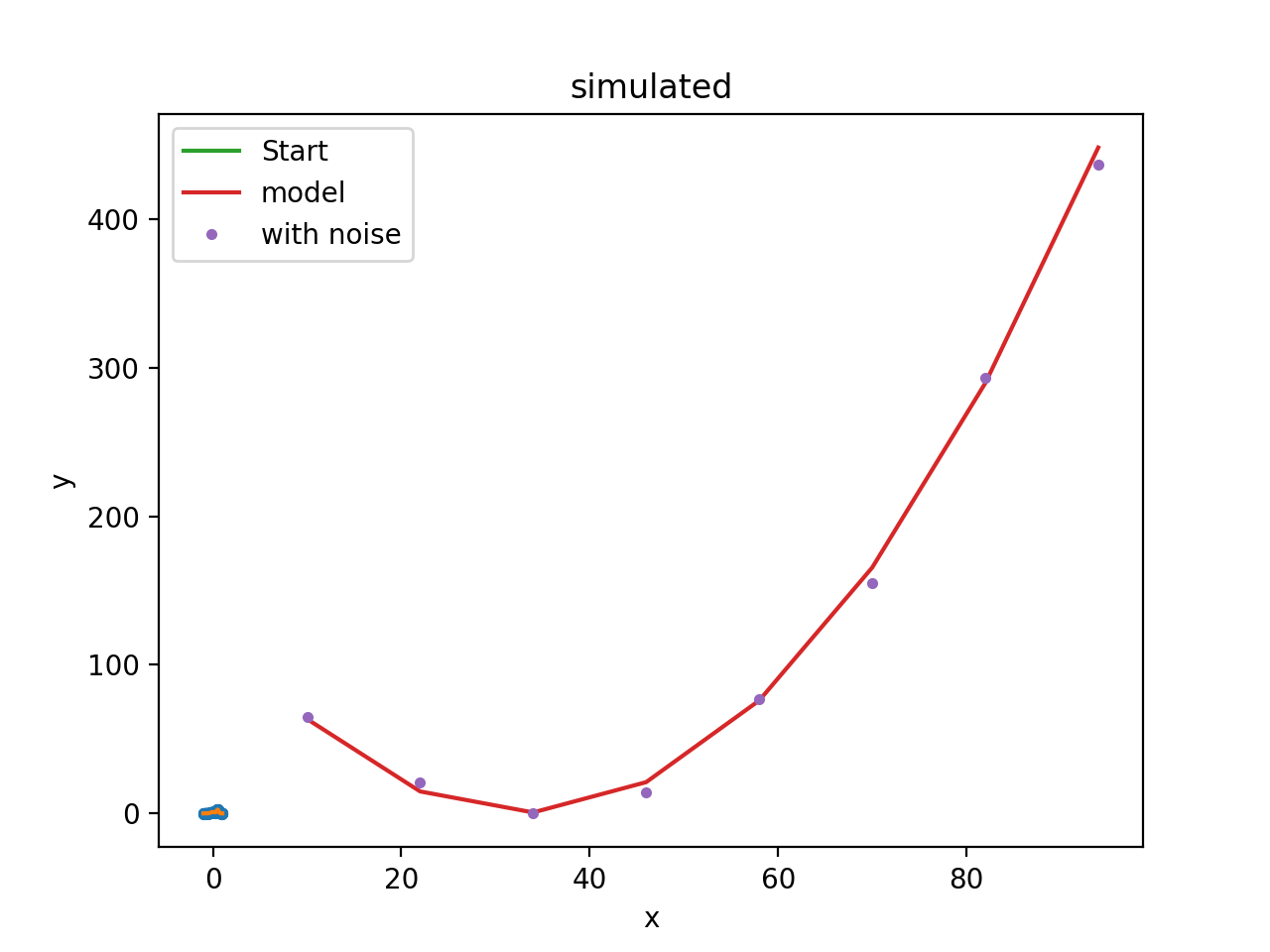
>>> ymdl = mdl(x)
>>> rng = np.random.default_rng(235)  # a "repeatable" set of random values
>>> from sherpa.utils import poisson_noise
>>> ypoisson = poisson_noise(ymdl, rng=rng)
>>> ypoisson = poisson_noise(ymdl, rng=rng)
>>> import matplotlib.pyplot as plt
>>> plt.plot(x, ymdl, label="model")
[<matplotlib.lines.Line2D object at ...>]
>>> plt.plot(x, ypoisson, ".", label="with noise")
[<matplotlib.lines.Line2D object at ...>]
>>> plt.legend()
<matplotlib.legend.Legend object at ...>

X-ray data (DataPHA)
In principle, the same steps apply when simulating PHA data
(DataPHA objects), however, the mechanics are a
little more complicated because we need to account for the
instrumental response (ARF and RMF) and possibly also
the background, which may contribute to the source spectrum that we
want to simulate. Readers not interested in X-ray data analysis may
want to skip this section.
Sherpa offers a dedicated function sherpa.astro.fake.fake_pha() for
simulations of PHA data. A DataPHA object
needs to be set up with the responses for the source and an exposure
time.
Usually, the easiest setup is to read in a PHA file from a real observation taken
in a configuration close to what we want to simulate. This PHA file
that already specifies the response and backgrounds so that they can be automatically
loaded. Also, the exposure time, background scaling etc. will be taken
from the header of the file, but we can change these values if we want.
When new data is simulated later, the counts in data will be overwritten,
but all other information stays the same.
In this example, we use a datafile from Sherpa’s test data files
(which are large and not installed by default
but can be downloaded).
>>> # Set the directory where the data is stored.
>>> # In this case, we use Sherpa's test data files
>>> from sherpa.utils.testing import get_datadir
>>> data_dir = get_datadir() + '/'
>>> # Load the data from a PHA file
>>> from sherpa.astro.io import read_pha
>>> data = read_pha(data_dir + '9774_bg.pi')
>>> data.exposure = 5e5  # Simulate longer exposure than in the original data
Alternatively, we first create a DataPHA object with
the correct channel numbers, responses, and exposure time. In this example, we
initially set the exposure time and then add the remaining information line by line:
>>> import numpy as np
>>> from sherpa.astro.io import read_arf, read_rmf
>>> from sherpa.astro.data import DataPHA
>>> data = DataPHA(name='any', channel=None, counts=None, exposure=10000.)
>>> data.set_arf(read_arf(data_dir + '9774.arf'))
>>> data.set_rmf(read_rmf(data_dir + '9774.rmf'))
>>> # By convention, channel numbers usually start at 1
>>> data.channel = np.arange(1, data.get_rmf().detchans + 1)
>>> data.counts = np.zeros_like(data.channel)
Next, we set up a model. In this case, we start with a powerlaw source where the slope and normalization of that powerlaw are already known, e.g. from the literature. We then add a weak emission line. Our simulation will show us if this emission line would be detectable in a real observation:
>>> from sherpa.models.basic import PowLaw1D, Gauss1D
>>> pl = PowLaw1D()
>>> line = Gauss1D()
>>> pl.gamma = 1.8
>>> pl.ampl = 2e-05
>>> line.pos = 6.7
>>> line.ampl = .0003
>>> line.fwhm = .1
>>> srcmdl = pl + line
We will need to wrap this model with the response (ARF and RMF), which takes care of converting from channels to energy:
>>> resp = data.get_full_response()
>>> full_model = resp(srcmdl)
>>> print(full_model)
apply_rmf(apply_arf(10000.0 * (powlaw1d + gauss1d)))
  Param        Type          Value          Min          Max      Units
  -----        ----          -----          ---          ---      -----
  powlaw1d.gamma thawed          1.8          -10           10
  powlaw1d.ref frozen            1 -3.40282e+38  3.40282e+38
  powlaw1d.ampl thawed        2e-05            0  3.40282e+38
  gauss1d.fwhm thawed          0.1  1.17549e-38  3.40282e+38
  gauss1d.pos  thawed          6.7 -3.40282e+38  3.40282e+38
  gauss1d.ampl thawed       0.0003 -3.40282e+38  3.40282e+38
The simplest case: Simulate the source spectrum only
With this model, it is now easy to run the simulation, which will
calculate the expected number of counts in each spectral channel
(where the number and width of the channels is given by the responses)
and then draw from a Poisson distribution with this expected
number. Thus, the simulated number of counts in each channel is always
an integer and includes Poisson noise - running
fake_pha() twice with identical settings will give
slightly different answers. With default settings, the input model is
convolved with the RMF and multiplied by the ARF, and properly scaled
for the exposure time.
>>> from sherpa.astro.fake import fake_pha
>>> fake_pha(data, full_model)
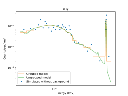
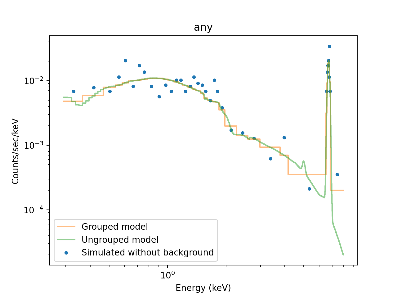
We bin the counts into bins of at least 5 counts per bin and display an image of the simulated spectrum (see X-ray data (DataPHA) for details):
>>> data.set_analysis('energy')
>>> data.notice(0.3, 8)
>>> data.group_counts(5)
>>> from sherpa.plot import DataPlot
>>> nobgplot = DataPlot()
>>> nobgplot.prepare(data)
We can overplot the model (both grouped and ungrouped):
>>> from sherpa.astro.plot import ModelPHAHistogram, ModelHistogram
>>> nobgplot.plot(xlog=True, ylog=True, label='Simulated without background')
>>> m1plot = ModelPHAHistogram()
>>> m1plot.prepare(data, full_model)
>>> m1plot.overplot(alpha=0.5, label="Grouped model")
>>> m2plot = ModelHistogram()
>>> m2plot.prepare(data, full_model)
>>> m2plot.overplot(alpha=0.5, label="Ungrouped model")

Sometimes, more than one response is needed, e.g. in Chandra LETG/HRC-S
different orders of the grating overlap on the detector, so they all
contribute to the observed source
spectrum.
The models that are passed into fake_pha()
can be arbitrarily complex and can contain multiple components. For example,
fake_pha() can simulate
models which may include such components as the instrumental
background (which should not be folded through the ARF) or arbitrary
other components:
>>> fake_pha(data, model=inst_bkg + resp(srcmodel))
Adding background
Weak spectral features can be hidden in a large (instrumental or astrophysical) background, thus it can be important to include background in the simulation.
Sample background from a PHA file
One way to include background is to sample it from a
DataPHA object. To do so, a background need to be
loaded into the dataset before running the simulation and, if not done
before, the scale of the background scaling has to be set:
>>> data.set_background(read_pha(data_dir + '9774_bg.pi'))
>>> data.backscal = 9.6e-06
>>> fake_pha(data, full_model)
>>> data.set_analysis('energy')
>>> data.notice(0.3, 8)
>>> data.group_counts(5)
>>> samplebgplot = DataPlot()
>>> samplebgplot.prepare(data)
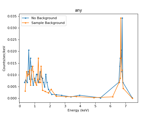
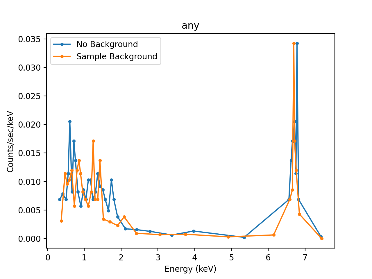
>>> nobgplot.plot(label='No Background',linestyle="solid")
>>> samplebgplot.plot(overplot=True, label='Sample Background', linestyle="solid")

The fake_pha function simulates the source spectrum as above, but
then it samples from the background PHA. For each bin, it treats the
background count number as the expected value and performs a Poisson
draw. The background drawn from the Poisson distribution is than added
to the simulated source spectrum (the sum of two Poisson distributions
is a Poisson distribution again). This works best if the background is
well exposed and has a large number or counts.
More than one background
If more than one background is set up, then the expected backgrounds will be averaged before the Poisson draw.
Background models
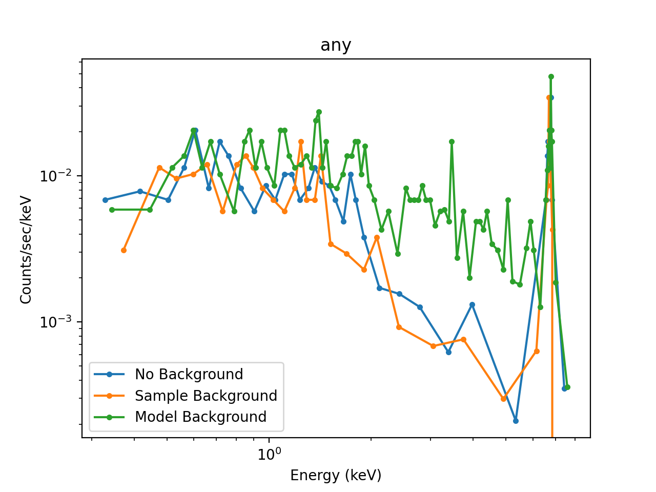
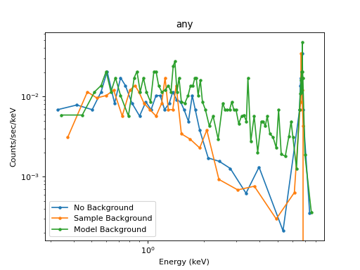
When the number of counts in the background is low, the above procedure amplifies the noise. The experimental background already contains noise just from Poisson statistics. Using the observed count numbers as background value and then performing a Poisson draw on them again gives a higher level of noise than a real observation would have. To avoid this problem, a background model may be used instead. In this example, we assume that the background is dominated by an astrophysical component, so it gets folded through the response:
>>> from sherpa.models.basic import Const1D
>>> bkgmdl = Const1D('bmdl')
>>> bkgmdl.c0 = 1e-5
>>> fake_pha(data, resp(srcmdl + bkgmdl))
>>> data.set_analysis('energy')
>>> data.notice(0.3, 8)
>>> data.group_counts(5)
>>> modelbgplot = DataPlot()
>>> modelbgplot.prepare(data)
>>> nobgplot.plot(xlog=True, ylog=True, label='No Background', linestyle="solid")
>>> samplebgplot.plot(overplot=True, label='Sample Background', linestyle="solid")
>>> modelbgplot.plot(overplot=True, label='Model Background', linestyle="solid")
Reference/API
Simulate PHA datasets
The fake_pha routine is used to create simulated
sherpa.astro.data.DataPHA data objects.
Functions
|
Simulate a PHA data set from a model. |