Examples
The following examples show the different ways that a model can be evaluated, for a range of situations. The direct method is often sufficient, but for more complex cases it can be useful to ask a data object to evaluate the model, particularly if you want to include instrumental responses, such as a RMF and ARF.
Evaluating a one-dimensional model directly
In the following example a one-dimensional gaussian is evaluated
on a grid of 5 points by
using the model object directly.
The first approach just calls the model with the evaluation
grid (here the array x),
which uses the parameter values as defined in the model itself:
>>> from sherpa.models.basic import Gauss1D
>>> gmdl = Gauss1D()
>>> gmdl.fwhm = 100
>>> gmdl.pos = 5050
>>> gmdl.ampl = 50
>>> x = [4800, 4900, 5000, 5100, 5200]
>>> y1 = gmdl(x)
The second uses the calc()
method, where the parameter values must be specified in the
call along with the grid on which to evaluate the model.
The order matches that of the parameters in the model, which can be
found from the
pars attribute of the model:
>>> [p.name for p in gmdl.pars]
['fwhm', 'pos', 'ampl']
>>> y2 = gmdl.calc([100, 5050, 100], x)
>>> y2 / y1
array([ 2.,  2.,  2.,  2.,  2.])
Since in this case the amplitude (the last parameter value) is twice
that used to create y1 the ratio is 2 for each bin.
Evaluating a 2D model to match a Data2D object
In the following example the model is evaluated on a grid
specified by a dataset, in this case a set of two-dimensional
points stored in a Data2D object.
First the data is set up (there are only four points
in this example to make things easy to follow).
>>> from sherpa.data import Data2D
>>> x0 = [1.0, 1.9, 2.4, 1.2]
>>> x1 = [-5.0, -7.0, 2.3, 1.2]
>>> y = [12.1, 3.4, 4.8, 5.2]
>>> twod = Data2D('data', x0, x1, y)
For demonstration purposes, the Box2D
model is used, which represents a rectangle (any points within the
xlow
to
xhi
and
ylow
to
yhi
limits are set to the
ampl
value, those outside are zero).
>>> from sherpa.models.basic import Box2D
>>> mdl = Box2D('mdl')
>>> mdl.xlow = 1.5
>>> mdl.xhi = 2.5
>>> mdl.ylow = -9.0
>>> mdl.yhi = 5.0
>>> mdl.ampl = 10.0
The coverage have been set so that some of the points are within the “box”, and so are set to the amplitude value when the model is evaluated.
>>> twod.eval_model(mdl)
array([  0.,  10.,   10.,   0.])
The eval_model() method evaluates
the model on the grid defined by the data set, so it is the same
as calling the model directly with these values:
>>> twod.eval_model(mdl) == mdl(x0, x1)
array([ True,  True,  True,  True])
The eval_model_to_fit() method
will apply any filter associated with the data before
evaluating the model. At this time there is no filter
so it returns the same as above.
>>> twod.eval_model_to_fit(mdl)
array([  0.,  10.,   10.,   0.])
Adding a simple spatial filter - that excludes one of
the points within the box - with
ignore() now results
in a difference in the outputs of
eval_model()
and
eval_model_to_fit(),
as shown below. The call to
get_indep()
is used to show the grid used by
eval_model_to_fit().
>>> twod.ignore(x0lo=2, x0hi=3, x1lo=0, x1hi=10)
>>> twod.eval_model(mdl)
array([  0.,  10.,   10.,   0.])
>>> twod.get_indep(filter=True)
(array([ 1. ,  1.9,  1.2]), array([-5. , -7. ,  1.2]))
>>> twod.eval_model_to_fit(mdl)
array([  0.,  10.,   0.])
X-ray data (DataPHA)
PHA data is more complicated than other data types in Sherpa
because of the need to convert between the units used by the model
(energy or wavelength) and the units of the data (channel). As a user
you will generally be thinking in keV or Angstroms, but the
DataPHA class has to convert to channel
units internally. The PHA data format is mainly used for
astronomical X-ray observatories, such as Chandra, XMM-Newton or about a dozen other missions.
First we will load in a PHA dataset, along with its response files (ARF and RMF), and have a look at how we can interrogate the object.
>>> from sherpa.astro.io import read_pha
>>> pha = read_pha( data_dir + '9774.pi')
We can see that the ARF, RMF, and a background dataset have automatically been loaded for us.
read ARF file .../9774.arf
read RMF file .../9774.rmf
read background file .../9774_bg.pi
Instead, ARF and RMF could be loaded manually - with
sherpa.astro.io.read_arf(), sherpa.astro.io.read_rmf(),
and sherpa.astro.io.read_pha() -
and set with set_arf(),
set_rmf(), and
set_background()
methods of the DataPHA class:
>>> pha
<DataPHA data set instance '.../9774.pi'>
>>> pha.get_background()
<DataPHA data set instance '.../9774_bg.pi'>
>>> pha.get_arf()
<DataARF data set instance '.../9774.arf'>
>>> pha.get_rmf()
<DataRMF data set instance '.../9774.rmf'>
This is a Chandra imaging-mode ACIS observation, as shown by header keywords defined by OGIP, and so it has 1024 channels:
>>> pha.header['INSTRUME']
'ACIS'
>>> pha.header['DETNAM']
'ACIS-23567'
>>> pha.channel.size
1024
The raw data is available from the
channel and
counts attributes, but
it is better to use the various methods, such as
get_indep() and
get_dep(), to
access the data.
PHA data generally requires filtering to exclude parts of the
data, so let’s pick a common energy range for ACIS data,
0.3 to 7 keV, and then use that range - which is indicated
by the mask attribute -
to ensure we only group the data within this range:
>>> pha.set_analysis('energy')
>>> pha.notice(0.3, 7)
>>> tabs = ~pha.mask
>>> pha.group_counts(20, tabStops=tabs)
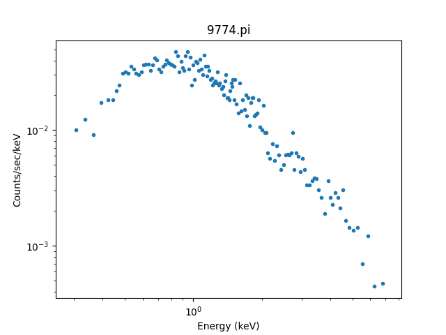
The standard Sherpa plotting setup can
be used to display the data. However we
have a PHA-specific class, DataPHAPlot,
which has better support for PHA data, as
discussed below:
>>> from sherpa.astro.plot import DataPHAPlot
>>> dplot = DataPHAPlot()
>>> dplot.prepare(pha)
>>> dplot.plot(xlog=True, ylog=True)
It can be useful to create these plots manually, so let’s step
through the steps. First we can access the data in channel
units using get_indep()
and get_dep(),
noting that get_indep returns a tuple so we want the
first element:
>>> chans, = pha.get_indep(filter=True)
>>> counts = pha.get_dep(filter=True)
>>> chans.size, counts.size
(460, 143)
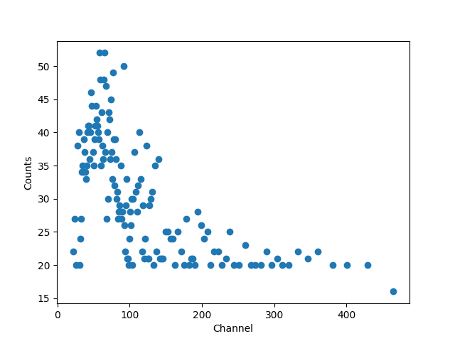
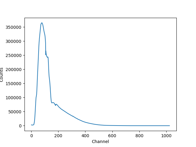
As shown above, the data sizes do not match. The counts has been grouped
while the channels data remains ungrouped. We can use the
apply_filter() method to
group the channel data, selecting the mid-point of each group, and
show the “raw” data (you can see that each group has at least
20 counts, except for the last one):
>>> gchans = pha.apply_filter(chans, pha._middle)
>>> gchans.size
143
>>> import matplotlib.pyplot as plt
>>> plt.clf()
>>> lines = plt.plot(gchans, counts, 'o')
>>> xlabel = plt.xlabel('Channel')
>>> ylabel = plt.ylabel('Counts')
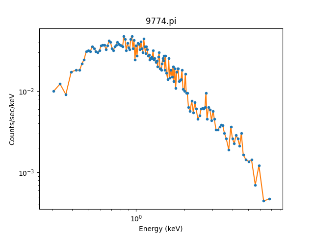
While the channel data is important, it doesn’t let us create
a plot like above. For this we
want to use the
get_x() and
get_y() methods,
which return data matching the analysis setting and,
for the dependent axis, normalizing by bin-width and
exposure time as appropriate. In this case we have selected
the “energy” setting so units are KeV for the X axis.
We can overplot the new data onto the previous plot to
show they match:
>>> x = pha.get_x()
>>> print(x.min(), x.max())
0.008030000200960785 14.943099975585938
>>> x = pha.apply_filter(x, pha._middle)
>>> y = pha.get_y(filter=True)
>>> dplot.plot(xlog=True, ylog=True)
>>> lines = plt.plot(x, y)
As mentioned, the DataPHAPlot class
handles the units for you. Switching the analysis setting
to wavelength will create a plot in Angstroms:
>>> pha.set_analysis('wave')
>>> print(pha.get_x().max())
1544.0122577477066
>>> from sherpa.plot import DataPlot
>>> wplot = DataPlot()
>>> wplot.prepare(pha)
>>> wplot.plot(linestyle='solid', xlog=True, ylog=True)
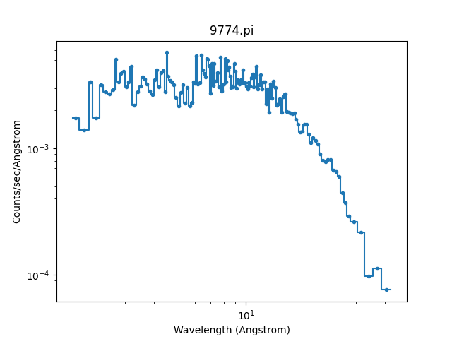
Note
By setting the linestyle option we get, along with a point
at the center of each group, a histogram-style line is drawn
indicating each group. Note that this is the major difference
to the sherpa.plot.DataPlot class, which would
just draw a line connecting the points.
For now we want to make sure we complete our analysis in energy units:
>>> pha.set_analysis('energy')
We can finally think about evaluating a model. To start with
we look at a physically-motivated model - an
absorbed (XSphabs)
powerlaw (PowLaw1D):
>>> from sherpa.models.basic import PowLaw1D
>>> from sherpa.astro.xspec import XSphabs
>>> pl = PowLaw1D()
>>> gal = XSphabs()
>>> mdl = gal * pl
>>> pl.gamma = 1.7
>>> gal.nh = 0.2
>>> print(mdl)
phabs * powlaw1d
   Param        Type          Value          Min          Max      Units
   -----        ----          -----          ---          ---      -----
   phabs.nH     thawed          0.2            0        1e+06 10^22 atoms / cm^2
   powlaw1d.gamma thawed          1.7          -10           10
   powlaw1d.ref frozen            1 -3.40282e+38  3.40282e+38
   powlaw1d.ampl thawed            1            0  3.40282e+38
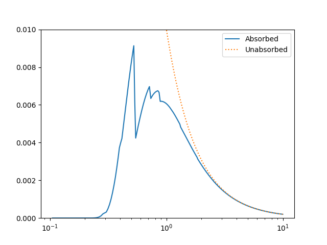
The model can be evaluated directly. XSPEC models use units of KeV for the X axis, so we generate a grid between 0.1 and 10 keV for use. As the data is binned we call the models - here the commbined model labelled “Absorbed” and just the powerlaw component labelled “Unabsorbed” - with both low and high edges:
>>> import numpy as np
>>> egrid = np.arange(0.1, 10, 0.01)
>>> elo, ehi = egrid[:-1], egrid[1:]
>>> emid = (elo + ehi) / 2
>>> plt.clf()
>>> lines = plt.plot(emid, mdl(elo, ehi), label='Absorbed')
>>> lines = plt.plot(emid, pl(elo, ehi), ':', label='Unabsorbed')
>>> plt.xscale('log')
>>> ylim = plt.ylim(0, 0.01)
>>> legend = plt.legend()
The Y axis has been restricted because the absorption is quite severe at low energies!
However, we need to include the response information -
ARF and RMF - in order to be able to
compare to the data. The easiest way to do this is to
use the Response1D
class to extract the ARF and RMF from the PHA dataset,
and then apply it to create a model expression, here
called full, which includes the corrections:
>>> from sherpa.astro.instrument import Response1D
>>> rsp = Response1D(pha)
>>> full = rsp(mdl)
>>> print(full)
apply_rmf(apply_arf(75141.227687398 * phabs * powlaw1d))
   Param        Type          Value          Min          Max      Units
   -----        ----          -----          ---          ---      -----
   phabs.nH     thawed          0.2            0        1e+06 10^22 atoms / cm^2
   powlaw1d.gamma thawed          1.7          -10           10
   powlaw1d.ref frozen            1 -3.40282e+38  3.40282e+38
   powlaw1d.ampl thawed            1            0  3.40282e+38
Note that the full model expression not only includes the
ARF and RMF terms, but also includes the exposure time of
the dataset. This ensures that the output has units of counts,
for XSPEC additive models whose normalization is per-second,
or defines the model amplitude to ber per-second, for models
such as PowLaw1D.
Note
Instead of using Response1D
you can directly create a model using
RSPModelPHA or
RSPModelNoPHA with logic
like
>>> from sherpa.astro.instrument import RSPModelPHA
>>> full = RSPModelPHA(arf, rmf, pha, pha.exposure * mdl)
Note that the exposure time is not automatically included for you as it
is with Response1D.
If we evaluate this model we get a surprise! The grid arguments are ignored (as long as something is sent in), and instead the model is evaluated on the channel group (hence the evaluated model as 1024 bins in this example):
>>> elo.size
989
>>> full(elo, ehi).size
1024
>>> full([1, 2, 3]).size
1024
>>> np.all(full(elo, ehi) == full([1, 2, 3]))
True
The evaluated model can therefore be displayed with a call such as:
>>> plt.clf()
>>> lines = plt.plot(pha.channel, full(pha.channel))
>>> xlabel = plt.xlabel('Channel')
>>> ylabel = plt.ylabel('Counts')
The reason for the ridiculously-large count range is because the powerlaw amplitude has not been changed from its default value of 1!
The eval_model() and
eval_model_to_fit() methods
can be used, but they must be applied to a response model
(e.g. full), otherwise the output will be meaningless:
>>> y1 = pha.eval_model(full)
>>> y2 = pha.eval_model_to_fit(full)
>>> y1.size, y2.size
(1024, 143)
The eval_model output is ungrouped whereas the
eval_model_to_fit output is grouped and filtered to
match the PHA dataset. In order to create a “nice” plot
we want to use energy units, which requires converting
between channel and energy units. For this we take advantage of
the data in the EBOUNDS extension of the RMF, which provides
an approximate mapping from channel to energy for visualization
purposes only. These arrays are available as the
e_min
and
e_max
attributes of the
DataRMF object returned by
get_rmf(), and we can
group them as we did earlier (except for choosing the
min and max labels for defining the bounds):
>>> rmf = pha.get_rmf()
>>> rmf.e_min.size, rmf.e_max.size
(1024, 1024)
>>> xlo = pha.apply_filter(rmf.e_min, pha._min)
>>> xhi = pha.apply_filter(rmf.e_max, pha._max)
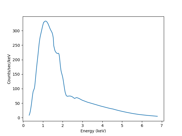
With these, we can convert the counts values returned by
eval_model_to_fit to counts per keV per second
(using the exposure
attribute to get the exposure time):
>>> x2 = pha.get_x()
>>> xmid = pha.apply_filter(x2, pha._middle)
>>> plt.clf()
>>> lines = plt.plot(xmid, y2 / (xhi - xlo) / pha.exposure)
>>> xlabel = plt.xlabel('Energy (keV)')
>>> ylable = plt.ylabel('Counts/sec/keV')
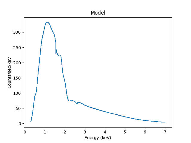
We can also use the Astronomy-specific
ModelHistogram plotting
class to display the model data without needing to
convert anything:
>>> from sherpa.astro.plot import ModelHistogram
>>> mplot = ModelHistogram()
>>> mplot.prepare(pha, full)
>>> mplot.plot()
The difference to the previous plot is that this one uses a histogram to display each bin while the previous version connected the mid-point of each bin (in this case the bins are small so it’s hard to see much difference).
We can use the model including the response to fit the data (here I am not going to tweak the statistic choice or optimiser which you should consider):
>>> from sherpa.fit import Fit
>>> fit = Fit(pha, full)
>>> res = fit.fit()
>>> print(res.format())
Method                = levmar
Statistic             = chi2gehrels
Initial fit statistic = 3.34091e+11
Final fit statistic   = 100.348 at function evaluation 37
Data points           = 143
Degrees of freedom    = 140
Probability [Q-value] = 0.995322
Reduced statistic     = 0.716768
Change in statistic   = 3.34091e+11
   phabs.nH       0.0129631    +/- 0.00727541
   powlaw1d.gamma   1.78432      +/- 0.0459914
   powlaw1d.ampl   7.17016e-05  +/- 2.48877e-06
We can see the amplitude has changed from 1 to \(\sim 10^{-4}\), which should make the predicted counts a lot more believable! We can display the data and model together:
>>> dplot.prepare(pha)
>>> dplot.plot(xlog=True)
>>> mplot2 = ModelHistogram()
>>> mplot2.prepare(pha, full)
>>> mplot2.overplot()
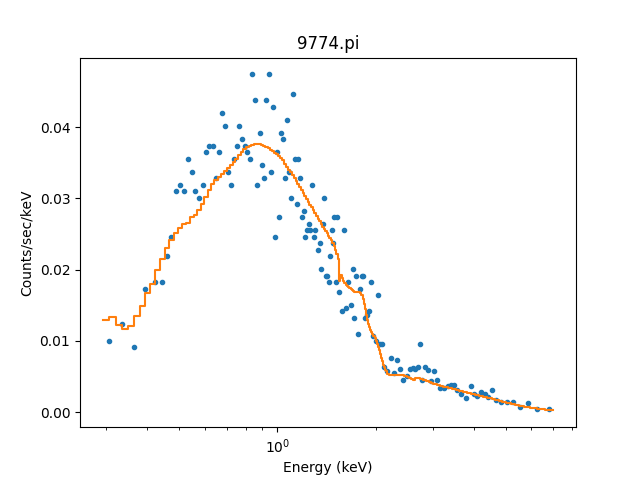
Note that this example has not tried to subtract the background or fit it!