Combining models and parameters
Most of the examples show far have used a single model component, such as a one-dimensional polynomial or a two-dimensional gaussian, but individual components can be combined, most commonly by addition, multiplication, subtraction, or even division. Components can also be combined with scalar values or - with great care - NumPy vectors. Parameter values can be “combined” by linking them together using mathematical expressions. The case of one model requiring the results of another model is discussed in the convolution section.
Model Expressions
A model, whether it is required to create a
sherpa.fit.Fit object or the argument to
the sherpa.ui.set_source() call, is expected to
behave like an instance of the
sherpa.models.model.ArithmeticModel class.
Instances can be combined as
numeric types
since the class defines methods for addition, subtraction,
multiplication, division, modulus, and exponentiation.
This means that Sherpa model instances can be combined with
other Python terms, such as the weighted combination of
model components cpt1, cpt2, and cpt3:
cpt1 * (cpt2 + 0.8 * cpt3)
Since the models are evaluated on a grid, it is possible to include a NumPy vector in the expression, but this is only possible in restricted situations, when the grid size is known (i.e. the model expression is not going to be used in a general setting).
Any ufunc can be used to combine models
Any universal function (“ufunc”) can be used to modify or combine models, for example:
>>> import numpy as np
>>> from sherpa.models import Gauss1D
>>> g1 = Gauss1D("g1")
>>> mdl = np.log10(g1)
This includes many commonly used mathematical and trigonometric functions
that are defines in the NumPy library,
such as log, exp, sin, cos, which allows building quite complex model expressions.
Only the numpy versions work here, not the functions from the
build-in math module, so use numpy.exp instead of math.exp.
Many more complex functions are available in
scipy.special;
any arbitrary Python function can be turned into a ufunc with
numpy.frompyfunc
and the interface is also available for
C extensions.
This allows a user to build quite complex model expressions, but in many cases it might be better to write a dedicated user model that encompasses that complexity.
In the following example, we combine two models, a Gaussian and a constant such that the resulting model value is always the maximum of the two:
>>> from sherpa.models import Const1D
>>> g1 = Gauss1D('g1')
>>> g1.fwhm = 2
>>> g1.ampl = 4
>>> c1 = Const1D('c1')
>>> c1.c0 = 1
>>> mdl = np.maximum(g1, c1)
>>> mdl(np.arange(-5, 5))
array([1., 1., 1., 1., 2., 4., 2., 1., 1., 1.])
Not every possible link function makes sense
With this flexibility, it is possible to define links that make no sense, for example taking the logical not of a parameter that represents a mass or turning values of parameters into arrays (Sherpa optimisers can only deal with scalar parameters). In practice, such mistakes are easy to spot when displaying a model; because Sherpa is meant to be a general and flexible modelling application that works with (almost) arbitrary user-defined models, the code puts as few restrictions as possible on the functions used for linking parameters.
Example
The following example fits two one-dimensional gaussians to a simulated dataset. It is based on the AstroPy modelling documentation, but has linked the positions of the two gaussians during the fit.
>>> import numpy as np
>>> import matplotlib.pyplot as plt
>>> from sherpa import data, models, stats, fit, plot
Since the example uses many different parts of the Sherpa API, the various modules are imported directly, rather than their contents, to make it easier to work out what each symbol refers to.
Note
Some Sherpa modules re-export symbols from other modules, which
means that a symbol can be found in several modules. An example
is sherpa.models.basic.Gauss1D, which can also be
imported as sherpa.models.Gauss1D.
Creating the simulated data
To provide a repeatable example, the NumPy random number generator is set to a fixed value:
>>> rng = np.random.default_rng(42)
The two components used to create the simulated dataset are called
sim1 and sim2:
>>> s1 = models.Gauss1D('sim1')
>>> s2 = models.Gauss1D('sim2')
The individual components can be displayed, as the __str__
method of the model class creates a display which includes the
model expression and then a list of the parameters:
>>> print(s1)
sim1
   Param        Type          Value          Min          Max      Units
   -----        ----          -----          ---          ---      -----
   sim1.fwhm    thawed           10  1.17549e-38  3.40282e+38
   sim1.pos     thawed            0 -3.40282e+38  3.40282e+38
   sim1.ampl    thawed            1 -3.40282e+38  3.40282e+38
The pars attribute contains
a tuple of all the parameters in a model instance. This can be
queried to find the attributes of the parameters (each element
of the tuple is a Parameter
object):
>>> [p.name for p in s1.pars]
['fwhm', 'pos', 'ampl']
These components can be combined using standard mathematical operations; for example addition:
>>> sim_model = s1 + s2
The sim_model object represents the sum of two gaussians, and
contains both the input models (using different names when creating
model components - so here sim1 and sim2 - can make it
easier to follow the logic of more-complicated model combinations):
>>> print(sim_model)
sim1 + sim2
   Param        Type          Value          Min          Max      Units
   -----        ----          -----          ---          ---      -----
   sim1.fwhm    thawed           10  1.17549e-38  3.40282e+38
   sim1.pos     thawed            0 -3.40282e+38  3.40282e+38
   sim1.ampl    thawed            1 -3.40282e+38  3.40282e+38
   sim2.fwhm    thawed           10  1.17549e-38  3.40282e+38
   sim2.pos     thawed            0 -3.40282e+38  3.40282e+38
   sim2.ampl    thawed            1 -3.40282e+38  3.40282e+38
The pars attribute now includes parameters from both components,
and so
the fullname
attribute is used to discriminate between the two components:
>>> [p.fullname for p in sim_model.pars]
['sim1.fwhm', 'sim1.pos', 'sim1.ampl', 'sim2.fwhm', 'sim2.pos', 'sim2.ampl']
Since the original models are still accessible, they can be used to
change the parameters of the combined model. The following sets the
first component (sim1) to be centered at x = 0 and the
second one at x = 0.5:
>>> s1.ampl = 1.0
>>> s1.pos = 0.0
>>> s1.fwhm = 0.5
>>> s2.ampl = 2.5
>>> s2.pos = 0.5
>>> s2.fwhm = 0.25
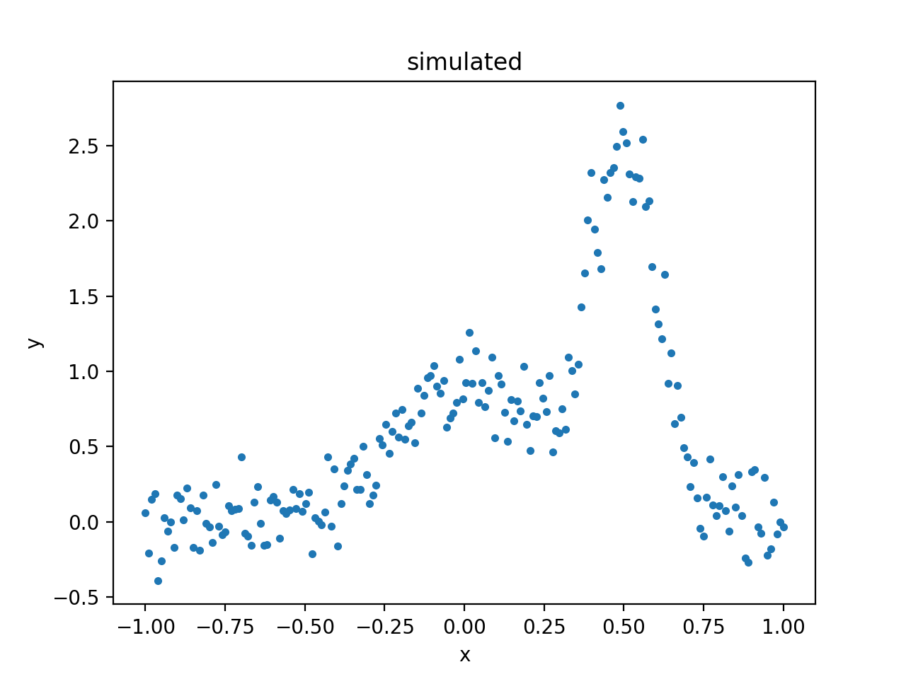
The model is evaluated on the grid, and “noise” added to it (using a normal distribution centered on 0 with a standard deviation of 0.2):
>>> x = np.linspace(-1, 1, 200)
>>> y = sim_model(x) + rng.normal(0., 0.2, x.shape)
These arrays are placed into a Sherpa data object, using the
Data1D class, since it will be fit
below, and then a plot created to show the simulated data:
>>> d = data.Data1D('simulated', x, y)
>>> dplot = plot.DataPlot()
>>> dplot.prepare(d)
>>> dplot.plot()

What is the composite model?
The result of the combination is a
BinaryOpModel, which has
op,
lhs,
and rhs
attributes which describe the structure of the combination:
>>> sim_model
<BinaryOpModel model instance 'sim1 + sim2'>
>>> sim_model.op
<ufunc 'add'>
>>> sim_model.lhs
<Gauss1D model instance 'sim1'>
>>> sim_model.rhs
<Gauss1D model instance 'sim2'>
There is also a
parts attribute
which contains all the elements of the model (in this case the
combination of the lhs and rhs attributes):
>>> sim_model.parts
(<Gauss1D model instance 'sim1'>, <Gauss1D model instance 'sim2'>)
>>> for cpt in sim_model.parts:
...     print(cpt)
sim1
   Param        Type          Value          Min          Max      Units
   -----        ----          -----          ---          ---      -----
   sim1.fwhm    thawed          0.5  1.17549e-38  3.40282e+38
   sim1.pos     thawed            0 -3.40282e+38  3.40282e+38
   sim1.ampl    thawed            1 -3.40282e+38  3.40282e+38
sim2
   Param        Type          Value          Min          Max      Units
   -----        ----          -----          ---          ---      -----
   sim2.fwhm    thawed         0.25  1.17549e-38  3.40282e+38
   sim2.pos     thawed          0.5 -3.40282e+38  3.40282e+38
   sim2.ampl    thawed          2.5 -3.40282e+38  3.40282e+38
As the BinaryOpModel class is a
subclass of the ArithmeticModel
class, the combined model can be treated as a single model instance;
for instance it can be evaluated on a grid by passing in an array of
values:
>>> sim_model([-1.0, 0, 1])
array([  1.52587891e-05,   1.00003815e+00,   5.34057617e-05])
In the example above, the model consists of two components sim1 and sim2
and we keep referencing them by their original variables. In general, more complex models
with more components can be built, which will then be arranged in a tree where the
leaves are the original components and the internal nodes are the either
BinaryOpModel (which combine two models) or
UnaryOpModel (with modify just one model on
the level below, e.g. by taking the absolute value of the output of the lower level model)
instances. Those models can be quite deep and thus Sherpa provides a syntax to access the
components of a model tree either by name or by model class. If more than one component
matches the name or class, a list of all matching components is returned:
>>> sim_model['sim2']
<Gauss1D model instance 'sim2'>
>>> sim_model[models.Gauss1D]
[<Gauss1D model instance 'sim1'>, <Gauss1D model instance 'sim2'>]
Setting up the model
Rather than use the model components used to simulate the data, new instances are created and combined to create the model:
>>> g1 = models.Gauss1D('g1')
>>> g2 = models.Gauss1D('g2')
>>> mdl = g1 + g2
In this particular fit, the separation of the two models is going
to be assumed to be known, so the two pos parameters can
be linked together, which means that there
is one less free parameter in the fit:
>>> g2.pos = g1.pos + 0.5
The FWHM parameters are changed as the default value of 10 is not appropriate for this data (since the independent axis ranges from -1 to 1):
>>> g1.fwhm = 0.1
>>> g2.fwhm = 0.1
The display of the combined model shows that the g2.pos
parameter is now linked to the g1.pos value:
>>> print(mdl)
g1 + g2
   Param        Type          Value          Min          Max      Units
   -----        ----          -----          ---          ---      -----
   g1.fwhm      thawed          0.1  1.17549e-38  3.40282e+38
   g1.pos       thawed            0 -3.40282e+38  3.40282e+38
   g1.ampl      thawed            1 -3.40282e+38  3.40282e+38
   g2.fwhm      thawed          0.1  1.17549e-38  3.40282e+38
   g2.pos       linked          0.5       expr: g1.pos + 0.5
   g2.ampl      thawed            1 -3.40282e+38  3.40282e+38
An alternative way to write the code above is to select the model components by name:
>>> mdl['g2'].fwhm = 0.1
While not necessary in this example, it can make it easier to keep track of a model with many components and simplify code that loops over model components. In the following example we want to built a model for the jet from a young star that has many separate emissions lines:
>>> spectral_lines = {'[O I]': 6300, 'Hα': 6563, '[N II]': 6586, '[S II]': 6716, '[S II]': 6731}
>>> jetlines = [models.Gauss1D(line) for line in spectral_lines.keys()]
>>> jetemission = models.Const1D('background') + np.sum(jetlines)
>>> for line, wave in spectral_lines.items():
...     jetemission[line].pos = wave
...     jetemission[line].fwhm = 0.1
>>> jetemission['Hα'].fwhm = 5.
Note
It is a good idea to check the parameter ranges - that is their minimum and maximum values - to make sure they are appropriate for the data.
The model is evaluated with its initial parameter values so that it can be compared to the best-fit location later:
>>> ystart = mdl(x)
Fitting the model
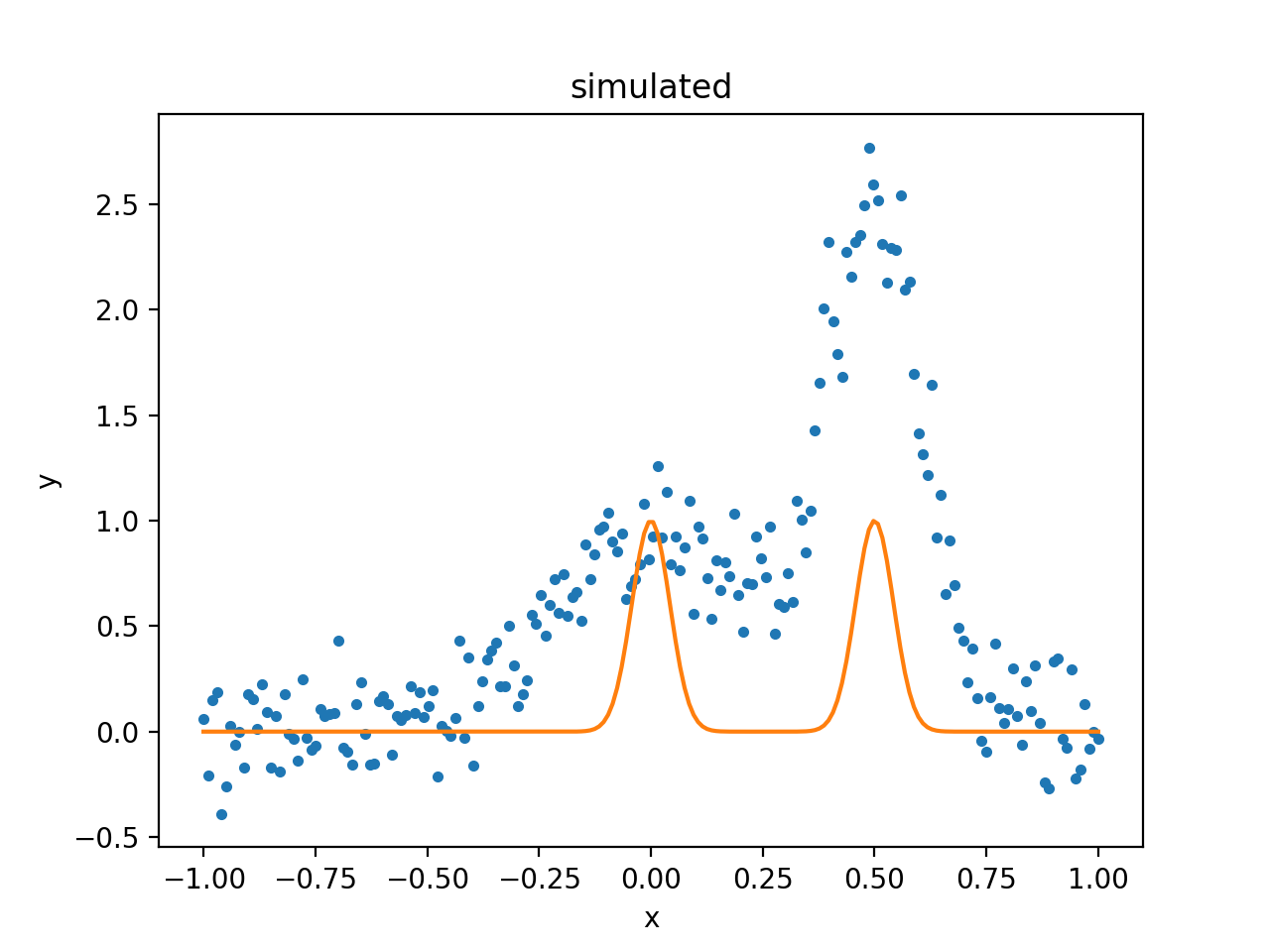
The initial model can be added to the data plot either directly,
with matplotlib commands, or using the
ModelPlot class to overlay onto the
DataPlot display:
>>> mplot = plot.ModelPlot()
>>> mplot.prepare(d, mdl)
>>> dplot.plot()
>>> mplot.plot(overplot=True)

As can be seen, the initial values for the gaussian positions are close to optimal. This is unlikely to happen in real-world situations!
As there are no errors for the data set, the least-square statistic
(LeastSq) is used (so that
the fit attempts to minimise the separation between the model and
data with no weighting), along with the default optimiser:
>>> f = fit.Fit(d, mdl, stats.LeastSq())
>>> res = f.fit()
>>> res.succeeded
True
When displaying the results, the FitPlot
class is used since it combines both data and model plots (after
updating the mplot object to include the new model parameter
values):
>>> fplot = plot.FitPlot()
>>> mplot.prepare(d, mdl)
>>> fplot.prepare(dplot, mplot)
>>> fplot.plot()
>>> _ = plt.plot(x, ystart, label='Start')
>>> _ = plt.legend(loc=2)
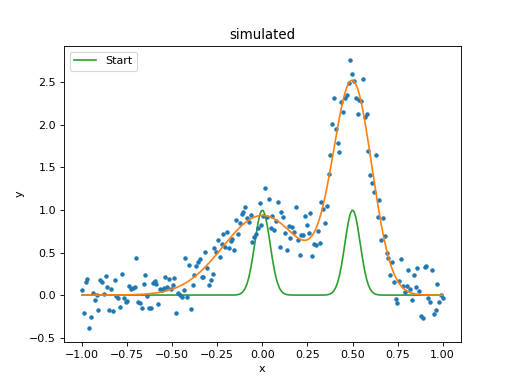
As can be seen below, the position of the g2 gaussian remains
linked to that of g1:
>>> print(mdl)
g1 + g2
   Param        Type          Value          Min          Max      Units
   -----        ----          -----          ---          ---      -----
   g1.fwhm      thawed     0.517499  1.17549e-38  3.40282e+38
   g1.pos       thawed  0.000168448 -3.40282e+38  3.40282e+38
   g1.ampl      thawed     0.935962 -3.40282e+38  3.40282e+38
   g2.fwhm      thawed     0.252366  1.17549e-38  3.40282e+38
   g2.pos       linked     0.500168       expr: g1.pos + 0.5
   g2.ampl      thawed       2.4535 -3.40282e+38  3.40282e+38
Accessing linked parameters
The pars attribute of a model instance provides access to the
individual Parameter objects.
These can be used to query - as shown below - or change the model
values:
>>> for p in mdl.pars:
...     if p.link is None:
...         print("{:10s} -> {:.3f}".format(p.fullname, p.val))
...     else:
...         print("{:10s} -> link to {}".format(p.fullname, p.link.name))
g1.fwhm    -> 0.517
g1.pos     -> 0.000
g1.ampl    -> 0.936
g2.fwhm    -> 0.252
g2.pos     -> link to g1.pos + 0.5
g2.ampl    -> 2.454
The linked parameter is actually an instance of the
CompositeParameter
class, which allows parameters to be combined in a similar
manner to models:
>>> g2.pos
<Parameter 'pos' of model 'g2'>
>>> print(g2.pos)
val         = 0.5001684477780305
min         = -3.4028234663852886e+38
max         = 3.4028234663852886e+38
units       =
frozen      = True
link        = g1.pos + 0.5
default_val = 0.5001684477780305
default_min = -3.4028234663852886e+38
default_max = 3.4028234663852886e+38
>>> g2.pos.link
<BinaryOpParameter 'g1.pos + 0.5'>
>>> print(g2.pos.link)
val         = 0.5001684477780305
min         = -3.4028234663852886e+38
max         = 3.4028234663852886e+38
units       =
frozen      = False
link        = None
default_val = 0.5001684477780305
default_min = -3.4028234663852886e+38
default_max = 3.4028234663852886e+38
What parameters are free to be fit?
When using an optimiser, it can be necessary to restrict the optimisation to a subset of the parameters of the model. Sherpa marks each parameter as frozen or thawed, where frozen parameters are not changed during a fit.
The frozen attribute of
a parameter can be read or written (or the
freeze() and
thaw() methods
can be used to change the setting):
>>> g1.fwhm.frozen
False
>>> g1.fwhm.frozen = True
The string display of a model indicates whether each parameter is
thawed, frozen, or linked under the Type column.
>>> print(mdl)
g1 + g2
   Param        Type          Value          Min          Max      Units
   -----        ----          -----          ---          ---      -----
   g1.fwhm      frozen     0.517499  1.17549e-38  3.40282e+38
   g1.pos       thawed  0.000168448 -3.40282e+38  3.40282e+38
   g1.ampl      thawed     0.935962 -3.40282e+38  3.40282e+38
   g2.fwhm      thawed     0.252366  1.17549e-38  3.40282e+38
   g2.pos       linked     0.500168       expr: g1.pos + 0.5
   g2.ampl      thawed       2.4535 -3.40282e+38  3.40282e+38
>>> g1.fwhm.frozen
True
>>> g1.fwhm.thaw()
Note that linked parameters are considered frozen even when the linked parameter is thawed:
>>> g2.pos.frozen
True
>>> print(g2.pos.link.fullname)
g1.pos + 0.5
>>> g1.pos.frozen
False
The freeze() and
thaw() methods can be used
to change the state for an individual parameter, and the
freeze() and
thaw() model versions will
change all the parameters of the model.
Note
Some parameters are marked as “always frozen”, such as the
ref parameter of the 1D
power law model, and these parameters can never be thawed.
How best to access the thawed parameters?
The thawedpars
attribute of a model will return the current numeric values of the
thawed parameters. It can also be used to change just the thawed
parameters, by setting it to a sequence of numbers (such as a NumPy
array or list).
>>> print(np.array(mdl.thawedpars))
[5.17498915e-01 1.68447778e-04 9.35962228e-01 2.52365591e-01
 2.45350047e+00]
>>> mdl.thawedpars = [0.1, 0.001, 1.0, 0.25, 2.5]
>>> print(mdl)
g1 + g2
   Param        Type          Value          Min          Max      Units
   -----        ----          -----          ---          ---      -----
   g1.fwhm      thawed          0.1  1.17549e-38  3.40282e+38
   g1.pos       thawed        0.001 -3.40282e+38  3.40282e+38
   g1.ampl      thawed            1 -3.40282e+38  3.40282e+38
   g2.fwhm      thawed         0.25  1.17549e-38  3.40282e+38
   g2.pos       linked        0.501       expr: g1.pos + 0.5
   g2.ampl      thawed          2.5 -3.40282e+38  3.40282e+38
The get_thawed_pars()
method will return the parameter objects representing the thawed
parameters:
>>> g1.get_thawed_pars()
[<Parameter 'fwhm' of model 'g1'>, <Parameter 'pos' of model 'g1'>, <Parameter 'ampl' of model 'g1'>]
>>> g2.get_thawed_pars()
[<Parameter 'fwhm' of model 'g2'>, <Parameter 'ampl' of model 'g2'>, <Parameter 'pos' of model 'g1'>]
>>> mdl.get_thawed_pars()
[<Parameter 'fwhm' of model 'g1'>, <Parameter 'pos' of model 'g1'>, <Parameter 'ampl' of model 'g1'>, <Parameter 'fwhm' of model 'g2'>, <Parameter 'ampl' of model 'g2'>]
Note
The thawed parameters of g2 include g1.pos, since it
is a linked parameter, but that the thawed parameters of mdl does
not end with this because it has already been included in the thawed
parameters from g1.
Warning
Do not try to use the values from the
pars attribute to determine
the free parameters in a model, since this attribute
does not include any linked parameters. For instance,
g2.pars does not reference g1.pos, even though
it is a free parameter:
>>> [m.fullname for m in g1.pars if not m.frozen]
['g1.fwhm', 'g1.pos', 'g1.ampl']
>>> [m.fullname for m in g2.pars if not m.frozen]
['g2.fwhm', 'g2.ampl']
The lpars attribute can be
used to find if there are any linked parameters in the model
that are not part of the model expression. So g2.lpars
will report g1.pos since the g1 model is not part of
to g2, but mdl.lpars will return nothing because it
contains the g1 component:
>>> g1.lpars
()
>>> g2.lpars
(<Parameter 'pos' of model 'g1'>,)
>>> mdl.lpars
()