Fitting the data
The Fit class takes the
data and model expression
to be fit, and uses the
optimiser to minimise the
chosen statistic. The basic
approach is to:
create a
Fitobject;call its
fit()method one or more times, potentially varying themethodattribute to change the optimiser;inspect the
FitResultsobject returned byfit()to extract information about the fit;review the fit quality, perhaps re-fitting with a different set of parameters or using a different optimiser;
once the “best-fit” solution has been found, calculate error estimates by calling the
est_errors()method, which returns aErrorEstResultsobject detailing the results;visualize the parameter errors with classes such as
IntervalProjectionandRegionProjection.
The following discussion uses a one-dimensional data set with gaussian errors (it was simulated with gaussian noise with \(\sigma = 5\)):
>>> import numpy as np
>>> import matplotlib.pyplot as plt
>>> from sherpa.data import Data1D
>>> d = Data1D('fit example', [-13, -5, -3, 2, 7, 12],
...            [102.3, 16.7, -0.6, -6.7, -9.9, 33.2],
...            np.ones(6) * 5)
It is going to be fit with the expression:
which is represented by the Polynom1D
model:
>>> from sherpa.models.basic import Polynom1D
>>> mdl = Polynom1D()
To start with, just the \(c_0\) and \(c_2\) terms are used in the fit:
>>> mdl.c2.thaw()
>>> print(mdl)
polynom1d
   Param        Type          Value          Min          Max      Units
   -----        ----          -----          ---          ---      -----
   polynom1d.c0 thawed            1 -3.40282e+38  3.40282e+38
   polynom1d.c1 frozen            0 -3.40282e+38  3.40282e+38
   polynom1d.c2 thawed            0 -3.40282e+38  3.40282e+38
   polynom1d.c3 frozen            0 -3.40282e+38  3.40282e+38
   polynom1d.c4 frozen            0 -3.40282e+38  3.40282e+38
   polynom1d.c5 frozen            0 -3.40282e+38  3.40282e+38
   polynom1d.c6 frozen            0 -3.40282e+38  3.40282e+38
   polynom1d.c7 frozen            0 -3.40282e+38  3.40282e+38
   polynom1d.c8 frozen            0 -3.40282e+38  3.40282e+38
   polynom1d.offset frozen            0 -3.40282e+38  3.40282e+38
Creating a fit object
A Fit object requires both a
data set and a
model object, and will use the
Chi2Gehrels
statistic with the
LevMar
optimiser
unless explicitly over-riden with the stat and
method parameters (when creating the object) or the
stat and
method attributes
(once the object has been created).
>>> from sherpa.fit import Fit
>>> f = Fit(d, mdl)
>>> print(f)
data      = fit example
model     = polynom1d
stat      = Chi2Gehrels
method    = LevMar
estmethod = Covariance
>>> print(f.data)
name      = fit example
x         = [-13, -5, -3, 2, 7, 12]
y         = [102.3, 16.7, -0.6, -6.7, -9.9, 33.2]
staterror = Float64[6]
syserror  = None
>>> print(f.model)
polynom1d
   Param        Type          Value          Min          Max      Units
   -----        ----          -----          ---          ---      -----
   polynom1d.c0 thawed            1 -3.40282e+38  3.40282e+38
   polynom1d.c1 thawed            0 -3.40282e+38  3.40282e+38
   polynom1d.c2 thawed            0 -3.40282e+38  3.40282e+38
   polynom1d.c3 frozen            0 -3.40282e+38  3.40282e+38
   polynom1d.c4 frozen            0 -3.40282e+38  3.40282e+38
   polynom1d.c5 frozen            0 -3.40282e+38  3.40282e+38
   polynom1d.c6 frozen            0 -3.40282e+38  3.40282e+38
   polynom1d.c7 frozen            0 -3.40282e+38  3.40282e+38
   polynom1d.c8 frozen            0 -3.40282e+38  3.40282e+38
   polynom1d.offset frozen            0 -3.40282e+38  3.40282e+38
The fit object stores references to objects, such as the model, which means that the fit object reflects the current state, and not just the values when it was created or used. For example, in the following the model is changed directly, and the value stored in the fit object is also changed:
>>> f.model.c2.val
0.0
>>> mdl.c2 = 1
>>> f.model.c2.val
1.0
Using the optimiser and statistic
With a Fit object can calculate the statistic value for
the current data and model
(calc_stat()),
summarise how well the current model represents the
data (calc_stat_info()),
calculate the per-bin chi-squared value (for chi-square
statistics; calc_stat_chisqr()),
fit the model to the data
(fit() and
simulfit()), and
calculate the parameter errors
(est_errors()).
>>> print("Starting statistic: {:.3f}".format(f.calc_stat()))
Starting statistic: 840.251
>>> sinfo1 = f.calc_stat_info()
>>> print(sinfo1)
name      =
ids       = None
bkg_ids   = None
statname  = chi2
statval   = 840.2511999999999
numpoints = 6
dof       = 4
qval      = 1.4661616529226985e-180
rstat     = 210.06279999999998
The fields in the StatInfoResults depend on
the choice of statistic; in particular,
rstat and
qval are set to None
if the statistic is not based on chi-square. The current data set
has a reduced statistic of \(\sim 200\) which indicates
that the fit is not very good (if the error bars in the
dataset are correct then a good fit is indicated by
a reduced statistic \(\simeq 1\) for
chi-square based statistics).
As with the model and statistic, if the data object is changed then
the results of calculations made on the fit object can be changed.
As shown below, when one data point is
removed, the calculated statistics
are changed (such as the
numpoints value).
>>> d.ignore(0, 5)
>>> sinfo2 = f.calc_stat_info()
>>> d.notice()
>>> sinfo1.numpoints
6
>>> sinfo2.numpoints
5
Note
The objects returned by the fit methods, such as
StatInfoResults and
FitResults, do not contain references
to any of the input objects. This means that the values stored
in these objects are not changed when the input values change.
The fit() method uses the optimiser to
vary the
thawed parameter values
in the model in an attempt to minimize the statistic value.
The method returns a
FitResults object which contains
information on the fit, such as whether it succeeded (found a minimum,
succeeded),
the start and end statistic value
(istatval and
statval),
and the best-fit parameter values
(parnames and
parvals).
>>> res = f.fit()
>>> if res.succeeded: print("Fit succeeded")
Fit succeeded
The return value has a format() method which
provides a summary of the fit:
>>> print(res.format())
Method                = levmar
Statistic             = chi2
Initial fit statistic = 840.251
Final fit statistic   = 96.8191 at function evaluation 6
Data points           = 6
Degrees of freedom    = 4
Probability [Q-value] = 4.67533e-20
Reduced statistic     = 24.2048
Change in statistic   = 743.432
   polynom1d.c0   -11.0742     +/- 2.91223
   polynom1d.c2   0.503612     +/- 0.0311568
The information is also available directly as fields of the
FitResults object:
>>> print(res)
datasets       = None
itermethodname = none
methodname     = levmar
statname       = chi2
succeeded      = True
parnames       = ('polynom1d.c0', 'polynom1d.c2')
parvals        = (-11.074165156709268, 0.5036124773506225)
statval        = 96.8190901009578
istatval       = 840.2511999999999
dstatval       = 743.4321098990422
numpoints      = 6
dof            = 4
qval           = 4.675333207707564e-20
rstat          = 24.20477252523945
message        = successful termination
nfev           = 6
The reduced chi square fit is now lower, \(\sim 25\), but still not close to 1.
Visualizing the fit
The DataPlot, ModelPlot,
and FitPlot classes can be used to
see how well the model represents the data.
>>> from sherpa.plot import DataPlot, ModelPlot
>>> dplot = DataPlot()
>>> dplot.prepare(f.data)
>>> mplot = ModelPlot()
>>> mplot.prepare(f.data, f.model)
>>> dplot.plot()
>>> mplot.overplot()
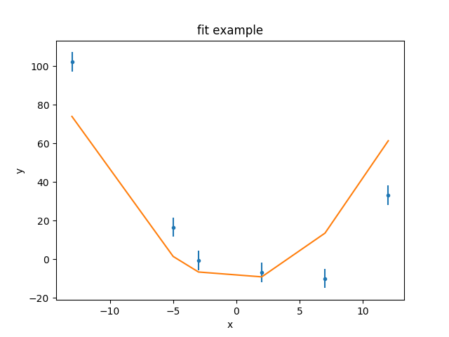
As can be seen, the model isn’t able to fully describe the data. One
check to make here is to change the optimiser in case the fit is stuck
in a local minimum. The default optimiser is
LevMar:
>>> f.method.name
'levmar'
>>> original_method = f.method
This can be changed to NelderMead
and the data re-fit.
>>> from sherpa.optmethods import NelderMead
>>> f.method = NelderMead()
>>> resn = f.fit()
In this case the statistic value has not changed, as shown by
dstatval being zero:
>>> print("Change in statistic: {}".format(resn.dstatval))
Change in statistic: 0.0
Note
An alternative approach is to create a new Fit object, with the
new method, and use that instead of changing the
method attribute. For instance:
>>> fit2 = Fit(d, mdl, method=NelderMead())
>>> fit2.fit()
Adjusting the model
This suggests that the problem is not that a local minimum has been found, but that the model is not expressive enough to represent the data. One possible approach is to change the set of points used for the comparison, either by removing data points - perhaps because they are not well calibrated or there are known to be issues - or adding extra ones (by removing a previously-applied filter). The approach taken here is to change the model being fit; in this case by allowing the linear term (\(c_1\)) of the polynomial to be fit, but a new model could have been tried.
>>> mdl.c1.thaw()
For the remainder of the analysis the original (Levenberg-Marquardt) optimiser will be used:
>>> f.method = original_method
With \(c_1\) allowed to vary, the fit finds a much better solution, with a reduced chi square value of \(\simeq 1.3\):
>>> res2 = f.fit()
>>> print(res2.format())
Method                = levmar
Statistic             = chi2
Initial fit statistic = 96.8191
Final fit statistic   = 4.01682 at function evaluation 8
Data points           = 6
Degrees of freedom    = 3
Probability [Q-value] = 0.259653
Reduced statistic     = 1.33894
Change in statistic   = 92.8023
   polynom1d.c0   -9.38489     +/- 2.91751
   polynom1d.c1   -2.41692     +/- 0.250889
   polynom1d.c2   0.478273     +/- 0.0312677
The previous plot objects can be used, but the model plot has to be
updated to reflect the new model values. Three new plot styles are used:
FitPlot shows both the data and model values,
DelchiPlot to show the residuals, and
SplitPlot to control the layout of the plots:
>>> from sherpa.plot import DelchiPlot, FitPlot, SplitPlot
>>> fplot = FitPlot()
>>> rplot = DelchiPlot()
>>> splot = SplitPlot()
>>> mplot.prepare(f.data, f.model)
>>> fplot.prepare(dplot, mplot)
>>> splot.addplot(fplot)
>>> rplot.prepare(f.data, f.model, f.stat)
>>> splot.addplot(rplot)
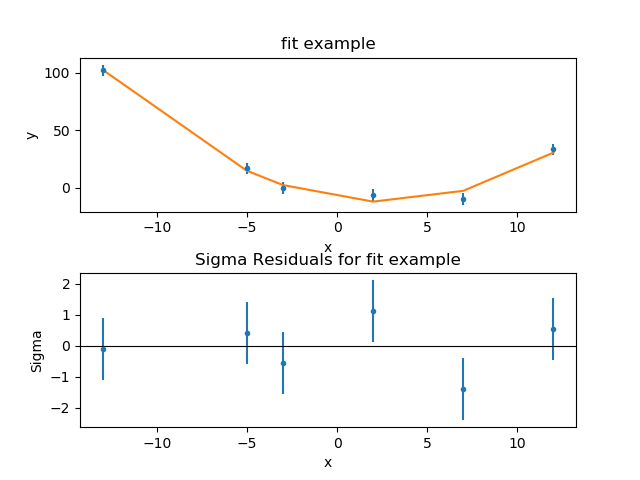
The residuals plot shows, on the ordinate, \(\sigma = (d - m) / e\) where \(d\), \(m\), and \(e\) are the data, model, and error value for each bin respectively.
The use of this style of plot - where there’s the data and fit
in the top and a related plot (normally some form of residual about
the fit) in the bottom - is common enough that Sherpa provides
a specialization of
SplitPlot called
JointPlot for this case. In the following
example the plots from above are re-used, as no settings have
changed, so there is no need to call the
prepare method of the component plots:
>>> from sherpa.plot import JointPlot
>>> jplot = JointPlot()
>>> jplot.plottop(fplot)
>>> jplot.plotbot(rplot)
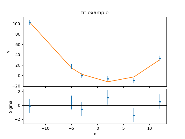
The two major changes to the SplitPlot output are that the
top plot is now taller, and the gap between the plots has
been reduced by removing the axis labelling from the first
plot and the title of the second plot (the X axes of the two
plots are also tied together, but that’s not obvious from this
example).
Refit from a different location
It may be useful to repeat the fit starting the model off at
different parameter locations to check that the fit solution is
robust. This can be done manually, or the
reset() method used to change
the parameters back to
the last values they were explicitly set to:
>>> mdl.reset()
Rather than print out all the components, most of which are fixed at
0, the first three can be looped over using the model’s
pars attribute:
>>> [(p.name, p.val, p.frozen) for p in mdl.pars[:3]]
[('c0', 1.0, False), ('c1', 0.0, False), ('c2', 1.0, False)]
There are many ways to choose the starting location; in this case the value of 10 is picked, as it is “far away” from the original values, but hopefully not so far away that the optimiser will not be able to find the best-fit location.
>>> for p in mdl.pars[:3]:
...     p.val = 10
...
Note
Since the parameter object - an instance of the
Parameter class - is being
accessed directly here, the value is changed via the
val attribute,
since it does not contain the same overloaded accessor functionality
that allows the setting of the parameter directly from the model.
The fields of the parameter object are:
>>> print(mdl.pars[1])
val         = 10.0
min         = -3.4028234663852886e+38
max         = 3.4028234663852886e+38
units       =
frozen      = False
link        = None
default_val = 10.0
default_min = -3.4028234663852886e+38
default_max = 3.4028234663852886e+38
How did the optimiser vary the parameters?
It can be instructive to see the “search path” taken by
the optimiser; that is, how the parameter values are changed per
iteration. The fit() method will write
these results to a file if the outfile parameter is set
(clobber is set here
to make sure that any existing file is overwritten):
>>> res3 = f.fit(outfile='fitpath.txt', clobber=True)
>>> print(res3.format())
Method                = levmar
Statistic             = chi2
Initial fit statistic = 196017
Final fit statistic   = 4.01682 at function evaluation 8
Data points           = 6
Degrees of freedom    = 3
Probability [Q-value] = 0.259653
Reduced statistic     = 1.33894
Change in statistic   = 196013
   polynom1d.c0   -9.38489     +/- 2.91751
   polynom1d.c1   -2.41692     +/- 0.250889
   polynom1d.c2   0.478273     +/- 0.0312677
The output file is a simple ASCII file where the columns give the function evaluation number, the statistic, and the parameter values:
# nfev statistic polynom1d.c0 polynom1d.c1 polynom1d.c2
0.000000e+00 1.960165e+05 1.000000e+01 1.000000e+01 1.000000e+01
1.000000e+00 1.960165e+05 1.000000e+01 1.000000e+01 1.000000e+01
2.000000e+00 1.960176e+05 1.000345e+01 1.000000e+01 1.000000e+01
3.000000e+00 1.960172e+05 1.000000e+01 1.000345e+01 1.000000e+01
4.000000e+00 1.961557e+05 1.000000e+01 1.000000e+01 1.000345e+01
5.000000e+00 4.016822e+00 -9.384890e+00 -2.416915e+00 4.782733e-01
6.000000e+00 4.016824e+00 -9.381649e+00 -2.416915e+00 4.782733e-01
7.000000e+00 4.016833e+00 -9.384890e+00 -2.416081e+00 4.782733e-01
8.000000e+00 4.016879e+00 -9.384890e+00 -2.416915e+00 4.784385e-01
9.000000e+00 4.016822e+00 -9.384890e+00 -2.416915e+00 4.782733e-01
As can be seen, a solution is found quickly in this situation. Is it the same as the previous attempt? Although the final statistic values are not the same, they are very close:
>>> res3.statval == res2.statval
False
>>> res3.statval - res2.statval
1.7763568394002505e-15
as are the parameter values:
>>> res2.parvals
(-9.384889507344186, -2.416915493735619, 0.4782733426100644)
>>> res3.parvals
(-9.384889507268973, -2.4169154937357664, 0.47827334260997567)
>>> for p2, p3 in zip(res2.parvals, res3.parvals):
...     print("{:+.2e}".format(p3 - p2))
...
+7.52e-11
-1.47e-13
-8.87e-14
The fact that the parameter values are very similar is good evidence for having found the “best fit” location, although this data set was designed to be easy to fit. Real-world examples often require more in-depth analysis.
Comparing models
Sherpa contains the calc_mlr() and
calc_ftest() routines which can be
used to compare the model fits (using the change in the
number of degrees of freedom and chi-square statistic) to
see if freeing up \(c_1\) is statistically meaningful.
>>> from sherpa.utils import calc_mlr
>>> calc_mlr(res.dof - res2.dof, res.statval - res2.statval)
5.778887632582094e-22
This provides evidence that the three-term model (with \(c_1\) free) is a statistically better fit, but the results of these routines should be reviewed carefully to be sure that they are valid; a suggested reference is Protassov et al. 2002, Astrophysical Journal, 571, 545.
Estimating errors
Note
Should I add a paragraph mentioning it can be a good idea to
rerun f.fit() to make sure any changes haven’t messsed up
the location?
There are two methods available to estimate errors from the fit object:
Covariance and
Confidence. The method to use can be set
when creating the fit object - using the estmethod parameter - or
after the object has been created, by changing the
estmethod attribute. The default method
is covariance
>>> print(f.estmethod.name)
covariance
which can be significantly faster faster, but less robust, than the confidence technique shown below.
The est_errors() method is used to calculate
the errors on the parameters and returns a
ErrorEstResults object:
>>> coverrs = f.est_errors()
>>> print(coverrs.format())
Confidence Method     = covariance
Iterative Fit Method  = None
Fitting Method        = levmar
Statistic             = chi2gehrels
covariance 1-sigma (68.2689%) bounds:
   Param            Best-Fit  Lower Bound  Upper Bound
   -----            --------  -----------  -----------
   polynom1d.c0     -9.38489     -2.91751      2.91751
   polynom1d.c1     -2.41692    -0.250889     0.250889
   polynom1d.c2     0.478273   -0.0312677    0.0312677
The EstErrResults object can also be displayed directly
(in a similar manner to the FitResults object returned
by fit):
>>> print(coverrs)
datasets    = None
methodname  = covariance
iterfitname = none
fitname     = levmar
statname    = chi2gehrels
sigma       = 1
percent     = 68.2689492137
parnames    = ('polynom1d.c0', 'polynom1d.c1', 'polynom1d.c2')
parvals     = (-9.384889507268973, -2.4169154937357664, 0.47827334260997567)
parmins     = (-2.917507940156572, -0.2508893171295504, -0.031267664298717336)
parmaxes    = (2.917507940156572, 0.2508893171295504, 0.031267664298717336)
nfits       = 0
The default is to calculate the one-sigma (68.3%) limits for
each thawed parameter. The
error range can be changed
with the
sigma attribute of the
error estimator, and the
set of parameters used in the
analysis can be changed with the parlist
attribute of the
est_errors()
call.
Warning
The error estimate should only be run when at a “good” fit. The
assumption is that the search statistic is chi-square distributed
so the change in statistic as a statistic varies can be related to
a confidence bound. One requirement is that - for chi-square
statistics - is that the reduced statistic value is small
enough. See the max_rstat field of the
EstMethod object.
Give the error if this does not happen (e.g. if c1 has not been fit)?
Changing the error bounds
The default is to calculate one-sigma errors, since:
>>> f.estmethod.sigma
1
This can be changed, e.g. to calculate 90% errors which are approximately \(\sigma = 1.6\):
>>> f.estmethod.sigma = 1.6
>>> coverrs90 = f.est_errors()
>>> print(coverrs90.format())
Confidence Method     = covariance
Iterative Fit Method  = None
Fitting Method        = levmar
Statistic             = chi2gehrels
covariance 1.6-sigma (89.0401%) bounds:
   Param            Best-Fit  Lower Bound  Upper Bound
   -----            --------  -----------  -----------
   polynom1d.c0     -9.38489     -4.66801      4.66801
   polynom1d.c1     -2.41692    -0.401423     0.401423
   polynom1d.c2     0.478273   -0.0500283    0.0500283
Note
As can be seen, 1.6 sigma isn’t quite 90%
>>> coverrs90.percent
89.0401416600884
Accessing the covariance matrix
The errors created by Covariance provides
access to the covariance matrix via the
extra_output attribute:
>>> print(coverrs.extra_output)
[[  8.51185258e+00  -4.39950074e-02  -6.51777887e-02]
 [ -4.39950074e-02   6.29454494e-02   6.59925111e-04]
 [ -6.51777887e-02   6.59925111e-04   9.77666831e-04]]
The order of these rows and columns matches that of the
parnames field:
>>> print([p.split('.')[1] for p in coverrs.parnames])
['c0', 'c1', 'c2']
Changing the estimator
The Confidence method takes each
thawed parameter and varies it until it finds the point where the
statistic has increased enough (the value is determined by the
sigma parameter and assumes the statistic is chi-squared
distributed). This is repeated separately for the upper and
lower bounds for each parameter. Since this can take time for
complicated fits, the default behavior is to display a message
when each limit is found (the
order these messages are displayed can change
from run to run):
>>> from sherpa.estmethods import Confidence
>>> f.estmethod = Confidence()
>>> conferrs = f.est_errors()
polynom1d.c0 lower bound:    -2.91751
polynom1d.c1 lower bound:    -0.250889
polynom1d.c0 upper bound:    2.91751
polynom1d.c2 lower bound:    -0.0312677
polynom1d.c1 upper bound:    0.250889
polynom1d.c2 upper bound:    0.0312677
As with the covariance run, the
return value is a ErrorEstResults object:
>>> print(conferrs.format())
Confidence Method     = confidence
Iterative Fit Method  = None
Fitting Method        = levmar
Statistic             = chi2gehrels
confidence 1-sigma (68.2689%) bounds:
   Param            Best-Fit  Lower Bound  Upper Bound
   -----            --------  -----------  -----------
   polynom1d.c0     -9.38489     -2.91751      2.91751
   polynom1d.c1     -2.41692    -0.250889     0.250889
   polynom1d.c2     0.478273   -0.0312677    0.0312677
Unlike the covariance errors, these are not guaranteed to be symmetrical (although in this example they are).
Using multiple cores
The example data and model used here does not require many
iterations to fit and calculate errors. However, for real-world
situations the error analysis can often take significantly-longer
than the fit. When using the
Confidence technique, the default
is to use all available CPU cores on the machine (the error range
for each parameter can be thought of as a separate task, and the
Python multiprocessing module is used to evaluate these tasks).
This is why the order of the
screen output from the
est_errors() call can vary.
The
parallel
attribute of the error estimator controls whether the
calculation should be run in parallel (True) or
not, and the
numcores attribute
determines how many CPU cores are used (the default is
to use all available cores).
>>> f.estmethod.name
'confidence'
>>> f.estmethod.parallel
True
The Covariance technique does not
provide a parallel option.
Using a subset of parameters
To save time, the error calculation can be restricted to a subset
of parameters by setting the parlist parameter of the
est_errors() call. As an example, the
errors on just \(c_1\) can be evaluated with the following:
>>> c1errs = f.est_errors(parlist=(mdl.c1, ))
polynom1d.c1 lower bound:    -0.250889
polynom1d.c1 upper bound:    0.250889
>>> print(c1errs)
datasets    = None
methodname  = confidence
iterfitname = none
fitname     = levmar
statname    = chi2gehrels
sigma       = 1
percent     = 68.26894921370858
parnames    = ('polynom1d.c1',)
parvals     = (-2.4169154937357664,)
parmins     = (-0.25088931712955054,)
parmaxes    = (0.25088931712955054,)
nfits       = 2
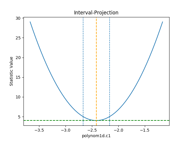
Visualizing the errors
The IntervalProjection class is used to
show how the statistic varies with a single parameter. It steps
through a range of values for a single parameter, fitting the
other thawed parameters, and displays the statistic value
(this gives an indication if the assumptions used to
calculate the errors
are valid):
>>> from sherpa.plot import IntervalProjection
>>> iproj = IntervalProjection()
>>> iproj.calc(f, mdl.c1)
>>> iproj.plot()
The default options display around one sigma from the best-fit
location (the range is estimated from the covariance error estimate).
The prepare() method is used
to change these defaults - e.g. by explicitly setting the min
and max values to use - or, as shown below, by scaling the
covariance error estimate using the fac argument:
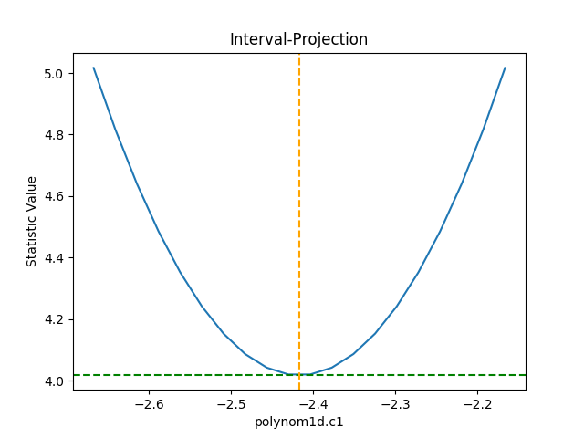
>>> iproj.prepare(fac=5, nloop=51)
The number of points has also been increased (the nloop argument)
to keep the curve smooth. Before re-plotting, the
calc()
method needs to be re-run to calculate the new data.
The one-sigma range is also added as vertical dotted
lines using
vline():
>>> iproj.calc(f, mdl.c1)
>>> iproj.plot()
>>> pmin = c1errs.parvals[0] + c1errs.parmins[0]
>>> pmax = c1errs.parvals[0] + c1errs.parmaxes[0]
>>> iproj.vline(pmin, overplot=True, linestyle='dot')
>>> iproj.vline(pmax, overplot=True, linestyle='dot')
Note
The vline()
method is a simple wrapper routine. Direct calls to
matplotlib can also be used to annotate the
visualization.
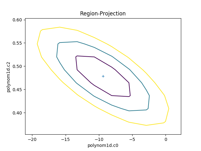
The RegionProjection class allows the
correlation between two parameters to be shown as a contour plot.
It follows a similar approach as
IntervalProjection, although the
final visualization is created with a call to
contour() rather than
plot:
>>> from sherpa.plot import RegionProjection
>>> rproj = RegionProjection()
>>> rproj.calc(f, mdl.c0, mdl.c2)
>>> rproj.contour()
The limits can be changed, either using the
fac parameter (as shown in the
interval-projection case), or
with the min and max parameters:
>>> rproj.prepare(min=(-22, 0.35), max=(3, 0.6), nloop=(41, 41))
>>> rproj.calc(f, mdl.c0, mdl.c2)
>>> rproj.contour()
>>> xlo, xhi = plt.xlim()
>>> ylo, yhi = plt.ylim()
>>> def get_limits(i):
...     return conferrs.parvals[i] + \
...            np.asarray([conferrs.parmins[i],
...                        conferrs.parmaxes[i]])
...
>>> plt.vlines(get_limits(0), ymin=ylo, ymax=yhi)
>>> plt.hlines(get_limits(2), xmin=xlo, xmax=xhi)
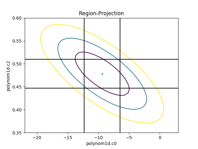
The vertical lines are added to indicate the one-sigma errors calculated by the confidence method earlier.
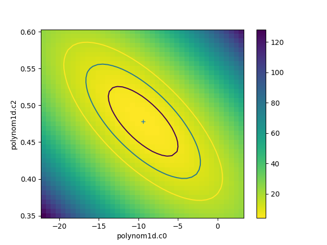
The calc call
sets the fields of the
RegionProjection object with the
data needed to create the plot. In the following example the
data is used to show the search statistic as an image, with the
contours overplotted. First, the axes of the image
are calculated (the extent argument to matplotlib’s
imshow command requires the pixel edges, not the
centers):
>>> xmin, xmax = rproj.x0.min(), rproj.x0.max()
>>> ymin, ymax = rproj.x1.min(), rproj.x1.max()
>>> nx, ny = rproj.nloop
>>> hx = 0.5 * (xmax - xmin) / (nx - 1)
>>> hy = 0.5 * (ymax - ymin) / (ny - 1)
>>> extent = (xmin - hx, xmax + hx, ymin - hy, ymax + hy)
The statistic data is stored as a one-dimensional array, and needs to be reshaped before it can be displayed:
>>> y = rproj.y.reshape((ny, nx))
>>> plt.clf()
>>> plt.imshow(y, origin='lower', extent=extent, aspect='auto', cmap='viridis_r')
>>> plt.colorbar()
>>> plt.xlabel(rproj.xlabel)
>>> plt.ylabel(rproj.ylabel)
>>> rproj.contour(overplot=True)
Simultaneous fits
Sherpa uses the
DataSimulFit and
SimulFitModel
classes to fit multiple data seta and models simultaneously.
This can be done explicitly, by combining individual data sets
and models into instances of these classes, or implicitly
with the simulfit() method.
It only makes sense to perform a simultaneous fit if there is some “link” between the various data sets or models, such as sharing one or model components or linking model parameters.
Poisson stats
Should there be something about using Poisson stats?