Comparing Gaussian, Lorentzian, and Voigt 1D models
Overview
In this example we will try to fit a peaked profile with a range of 1D models. If you have read the lmfit documentation then this example should seem familiar!
Setting up
The following sections will load in classes from Sherpa as needed, but it is assumed that the following module has been loaded:
>>> import matplotlib.pyplot as plt
Loading the data
The data can be retrieved from the
lmfit GitHub page.
It is a two-column ASCII file that can
be read in with NumPy or the sherpa.io.read_data()
routine:
>>> from sherpa.io import read_data
>>> d = read_data('test_peak.dat')
>>> print(d)
name      = test_peak.dat
x         = Float64[401]
y         = Float64[401]
staterror = None
syserror  = None
None
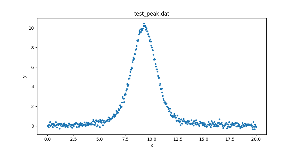
This could be displayed with matplotlib directly, but let’s create
a DataPlot to display it:
>>> from sherpa.plot import DataPlot
>>> dplot = DataPlot()
>>> dplot.prepare(d)
>>> dplot.plot()
Setting up the fits
We can then fit this with a variety of models, using the
LeastSq statistic and
NelderMead optimiser.
For each model -
NormGauss1D,
Lorentz1D,
PseudoVoigt1D,
and
Voigt1D - we create a
Fit instance:
>>> from sherpa.models.basic import NormGauss1D
>>> from sherpa.astro.models import Lorentz1D, PseudoVoigt1D, Voigt1D
>>> from sherpa.stats import LeastSq
>>> from sherpa.optmethods import NelderMead
>>> from sherpa.fit import Fit
>>> models = [NormGauss1D, Lorentz1D, PseudoVoigt1D, Voigt1D]
>>> stat = LeastSq()
>>> method = NelderMead()
>>> fits = {}
>>> for model in models:
...     mdl = model()
...     fit = Fit(d, mdl, stat, method)
...     fits[mdl.name] = fit
The fits dictionary is indexed by the model name which, in
this case, uses the default model names (as none were given when
initializing the model), which is the lower-case value of the
model. So the keys are 'normgauss1d', 'lorentz1d',
'pseudovoigt1d', and 'voigt1d'.
Fitting the NormGauss1D and Lorentz1D models
The fits could have been done in this loop, but let’s run them
separately. First the NormGauss1D and Lorentz1D models,
which bracket the data, using the
format() method to
display the fit results:
>>> result = fits['normgauss1d'].fit()
>>> print(result.format())
Method                = neldermead
Statistic             = leastsq
Initial fit statistic = 4222.73
Final fit statistic   = 29.9943 at function evaluation 439
Data points           = 401
Degrees of freedom    = 398
Change in statistic   = 4192.74
   normgauss1d.fwhm   2.90157
   normgauss1d.pos   9.24277
   normgauss1d.ampl   30.3135
>>> result = fits['lorentz1d'].fit()
>>> print(result.format())
Method                = neldermead
Statistic             = leastsq
Initial fit statistic = 4213.59
Final fit statistic   = 53.7535 at function evaluation 401
Data points           = 401
Degrees of freedom    = 398
Change in statistic   = 4159.84
   lorentz1d.fwhm   2.30967
   lorentz1d.pos   9.24439
   lorentz1d.ampl   38.9727
For reference, these results are essentially the same as obtained by lmfit.
We can create ModelPlot objects for each
model (extracting the model from the fit structure as I forgot to
save it earlier):
>>> from sherpa.plot import ModelPlot
>>> mplot1 = ModelPlot()
>>> mplot2 = ModelPlot()
>>> mplot1.prepare(d, fits['normgauss1d'].model)
>>> mplot2.prepare(d, fits['lorentz1d'].model)
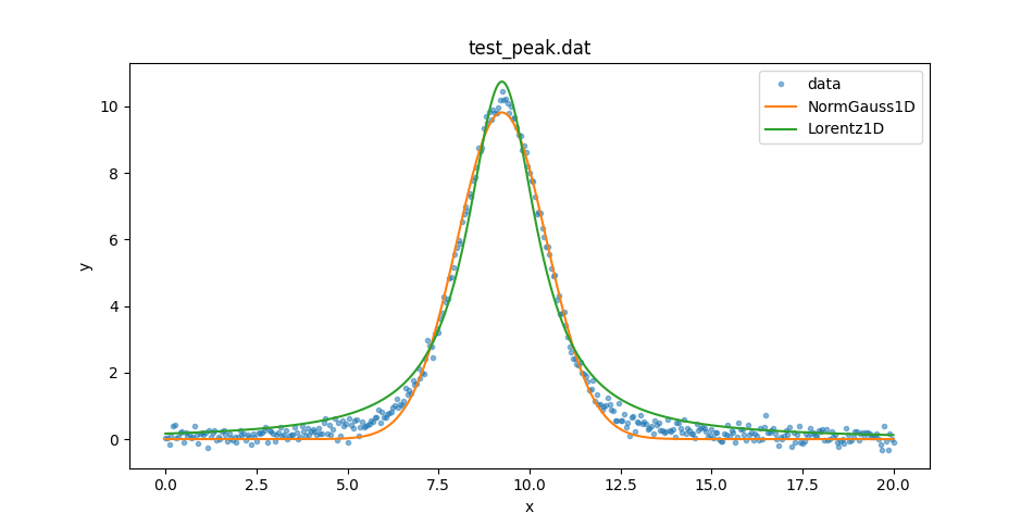
These can be used to compare the two model plots (I added in some matplotlib commands to set the plot legend):
>>> dplot.plot(alpha=0.5)
>>> ax = plt.gca()
>>> ax.lines[-1].set_label('data')
>>> mplot1.overplot()
>>> ax.lines[-1].set_label('NormGauss1D')
>>> mplot2.overplot()
>>> ax.lines[-1].set_label('Lorentz1D')
>>> plt.legend()
Fitting the PseudoVoigt1D and Voigt1D models
So neither model describe the data at the peak or the wings. Let’s
see if the extra freedom given by the PseudoVoigt1D and Voigt1D
models can help:
>>> result = fits['pseudovoigt1d'].fit()
>>> print(result.format())
Method                = neldermead
Statistic             = leastsq
Initial fit statistic = 4220.01
Final fit statistic   = 10.8366 at function evaluation 851
Data points           = 401
Degrees of freedom    = 397
Change in statistic   = 4209.18
   pseudovoigt1d.frac   0.533597
   pseudovoigt1d.fwhm   2.71357
   pseudovoigt1d.pos   9.2436
   pseudovoigt1d.ampl   34.4984
The Voigt1D fit here should be compared to the “gamma unconstrained”
version from the lmfit example.
>>> result = fits['voigt1d'].fit()
>>> print(result.format())
Method                = neldermead
Statistic             = leastsq
Initial fit statistic = 4211.75
Final fit statistic   = 10.9302 at function evaluation 738
Data points           = 401
Degrees of freedom    = 397
Change in statistic   = 4200.82
   voigt1d.fwhm_g   2.10801
   voigt1d.fwhm_l   1.0508
   voigt1d.pos    9.24375
   voigt1d.ampl   34.1915
The first thing to note is that the final statistic value, \(\sim 11\),
is much lower than either of the previous models, so they should be
a better fit, and that the PseudoVoigt1D model is “better” than
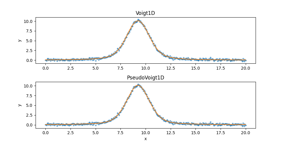
the Voigt1D model, but not by much. Since the two models appear
similar let’s create two plots:
>>> from sherpa.plot import SplitPlot
>>> mplot3 = ModelPlot()
>>> mplot4 = ModelPlot()
>>> mplot3.prepare(d, fits['voigt1d'].model)
>>> mplot4.prepare(d, fits['pseudovoigt1d'].model)
>>> splot = SplitPlot()
>>> splot.addplot(dplot, alpha=0.5)
>>> splot.overlayplot(mplot3)
>>> ax = plt.gca()
>>> ax.set_title('Voigt1D')
>>> ax.set_xlabel('')
>>> splot.addplot(dplot, alpha=0.5)
>>> splot.overlayplot(mplot4)
>>> ax = plt.gca()
>>> ax.set_title('PseudoVoigt1D')
Comparing the models
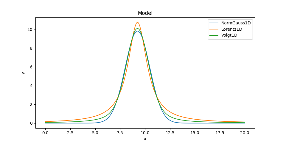
We can also overlay the models (here only showing one of the Voigt profiles since on this plot they appear identical):
>>> mplot1.plot()
>>> ax = plt.gca()
>>> ax.lines[-1].set_label('NormGauss1D')
>>> mplot2.overplot()
>>> ax.lines[-1].set_label('Lorentz1D')
>>> mplot3.overplot()
>>> ax.lines[-1].set_label('Voigt1D')
>>> plt.legend()