A quick guide to modeling and fitting in Sherpa
Here are some examples of using Sherpa to model and fit data. It is based on some of the examples used in the astropy.modelling documentation.
Getting started
The following modules are assumed to have been imported:
>>> import numpy as np
>>> import matplotlib.pyplot as plt
The basic process, which will be followed below, is:
Although presented as a list, it is not necessarily a linear process, in that the order can be different to that above, and various steps can be repeated. The above list also does not include any visualization steps needed to inform and validate any choices.
Fitting a one-dimensional data set
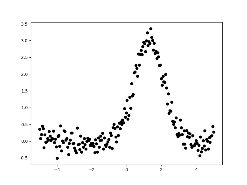
The following data - where x is the independent axis and
y the dependent one - is used in this example:
>>> np.random.seed(0)
>>> x = np.linspace(-5., 5., 200)
>>> ampl_true = 3
>>> pos_true = 1.3
>>> sigma_true = 0.8
>>> err_true = 0.2
>>> y = ampl_true * np.exp(-0.5 * (x - pos_true)**2 / sigma_true**2)
>>> y += np.random.normal(0., err_true, x.shape)
>>> plt.plot(x, y, 'ko');
The aim is to fit a one-dimensional gaussian to this data and to recover
estimates of the true parameters of the model, namely the position
(pos_true), amplitude (ampl_true), and width (sigma_true).
The err_true term adds in random noise (using a
Normal distribution)
to ensure the data is not perfectly-described by the model.
Creating a data object
Rather than pass around the arrays to be fit, Sherpa has the
concept of a “data object”, which stores the independent and dependent
axes, as well as any related metadata. For this example, the
class to use is Data1D, which requires
a string label (used to identify the data), the independent
axis, and then dependent axis:
>>> from sherpa.data import Data1D
>>> d = Data1D('example', x, y)
>>> print(d)
name      = example
x         = Float64[200]
y         = Float64[200]
staterror = None
syserror  = None
At this point no errors are being used in the fit, so the staterror
and syserror fields are empty. They can be set either when the
object is created or at a later time.
Plotting the data
The sherpa.plot module provides a number of classes that
create pre-canned plots. For example, the
sherpa.plot.DataPlot class can be used to display the data.
The steps taken are normally:
create the object;
call the
prepare()method with the appropriate arguments, in this case the data object;and then call the
plot()method.
Sherpa has one plotting backend, matplotlib, which is used to display plots. There is limited support for customizing these plots - such as always drawing the Y axis with a logarithmic scale - but extensive changes will require calling the plotting back-end directly.
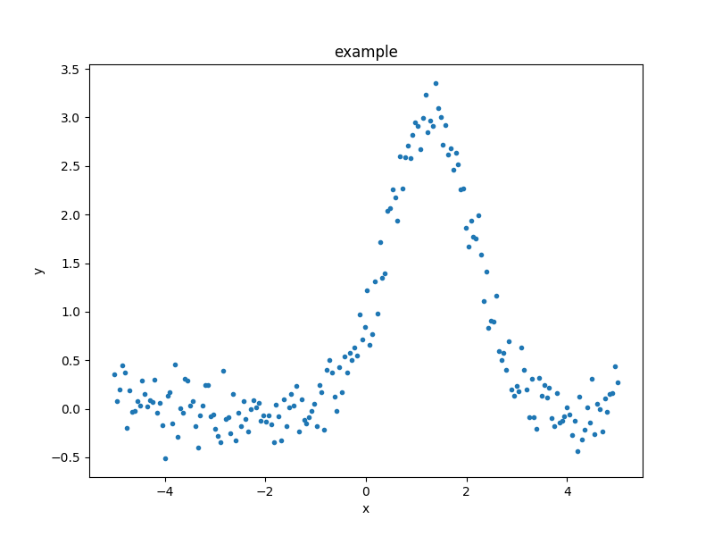
As an example of the DataPlot output:
>>> from sherpa.plot import DataPlot
>>> dplot = DataPlot()
>>> dplot.prepare(d)
>>> dplot.plot()
It is not required to use these classes and in the following, plots will be created either via these classes or directly via matplotlib.
Define the model
In this example a single model is used - a one-dimensional
gaussian provided by the Gauss1D
class - but more complex examples are possible: these
include multiple components,
sharing models between data sets, and
adding user-defined models.
A full description of the model language and capabilities is provided in
Creating model instances:
>>> from sherpa.models.basic import Gauss1D
>>> g = Gauss1D()
>>> print(g)
gauss1d
   Param        Type          Value          Min          Max      Units
   -----        ----          -----          ---          ---      -----
   gauss1d.fwhm thawed           10  1.17549e-38  3.40282e+38
   gauss1d.pos  thawed            0 -3.40282e+38  3.40282e+38
   gauss1d.ampl thawed            1 -3.40282e+38  3.40282e+38
It is also possible to restrict the range of a parameter, toggle parameters so that they are fixed or fitted, and link parameters together.
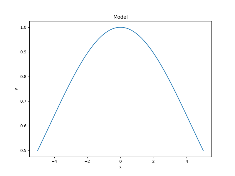
The sherpa.plot.ModelPlot class can be used to visualize
the model. The prepare() method
takes both a data object and the model to plot:
>>> from sherpa.plot import ModelPlot
>>> mplot = ModelPlot()
>>> mplot.prepare(d, g)
>>> mplot.plot()
There is also a sherpa.plot.FitPlot class which will
combine the two plot results,
but it is often just-as-easy to combine them directly:
>>> dplot.plot()
>>> mplot.overplot()
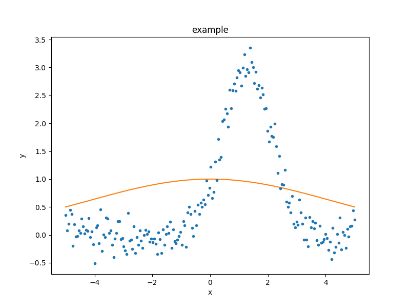
The model parameters can be changed - either manually or automatically - to try and start the fit off closer to the best-fit location, but for this example we shall leave the initial parameters as they are.
Select the statistics
In order to optimise a model - that is, to change the model parameters until the best-fit location is found - a statistic is needed. The statistic calculates a numerical value for a given set of model parameters; this is a measure of how well the model matches the data, and can include knowledge of errors on the dependent axis values. The optimiser (chosen below) attempts to find the set of parameters which minimises this statistic value.
For this example, since the dependent axis (y)
has no error estimate, we shall pick the least-square statistic
(LeastSq), which calculates the
numerical difference of the model to the data for each point:
>>> from sherpa.stats import LeastSq
>>> stat = LeastSq()
Select the optimisation routine
The optimiser is the part that determines how to minimise the statistic
value (i.e. how to vary the parameter values of the model to find
a local minimum). The main optimisers provided by Sherpa are
NelderMead
(also known as Simplex) and
LevMar
(Levenberg-Marquardt). The latter is often quicker, but less robust,
so we start with it (the optimiser can be changed and the data re-fit):
>>> from sherpa.optmethods import LevMar
>>> opt = LevMar()
>>> print(opt)
name    = levmar
ftol    = 1.19209289551e-07
xtol    = 1.19209289551e-07
gtol    = 1.19209289551e-07
maxfev  = None
epsfcn  = 1.19209289551e-07
factor  = 100.0
verbose = 0
Fit the data
The Fit class is used to bundle up the
data, model, statistic, and optimiser choices. The
fit() method runs the optimiser, and
returns a
FitResults instance, which
contains information on how the fit performed. This
infomation includes the
succeeded
attribute, to determine whether the fit converged, as well
as information on the fit (such as the start and end
statistic values) and best-fit parameter values. Note that
the model expression can also be queried for the new
parameter values.
>>> from sherpa.fit import Fit
>>> gfit = Fit(d, g, stat=stat, method=opt)
>>> print(gfit)
data      = example
model     = gauss1d
stat      = LeastSq
method    = LevMar
estmethod = Covariance
To actually fit the data, use the
fit() method, which - depending
on the data, model, or statistic being used - can take some
time:
>>> gres = gfit.fit()
>>> print(gres.succeeded)
True
One useful method for interactive analysis is
format(), which returns
a string representation of the fit results, as shown below:
>>> print(gres.format())
Method                = levmar
Statistic             = leastsq
Initial fit statistic = 180.71
Final fit statistic   = 8.06975 at function evaluation 30
Data points           = 200
Degrees of freedom    = 197
Change in statistic   = 172.641
   gauss1d.fwhm   1.91572      +/- 0.165982
   gauss1d.pos    1.2743       +/- 0.0704859
   gauss1d.ampl   3.04706      +/- 0.228618
Note
The LevMar optimiser calculates the
covariance matrix at the best-fit location, and the errors from
this are reported in the output from the call to the
fit() method. In this particular case -
which uses the LeastSq statistic -
the error estimates do not have much meaning. As discussed
below, Sherpa can make use of error estimates
on the data
to calculate meaningful parameter errors.
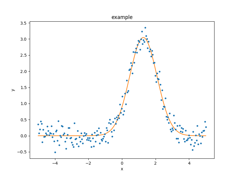
The sherpa.plot.FitPlot class will display the data
and model. The prepare() method
requires data and model plot objects; in this case the previous
versions can be re-used, although the model plot needs to be
updated to reflect the changes to the model parameters:
>>> from sherpa.plot import FitPlot
>>> fplot = FitPlot()
>>> mplot.prepare(d, g)
>>> fplot.prepare(dplot, mplot)
>>> fplot.plot()
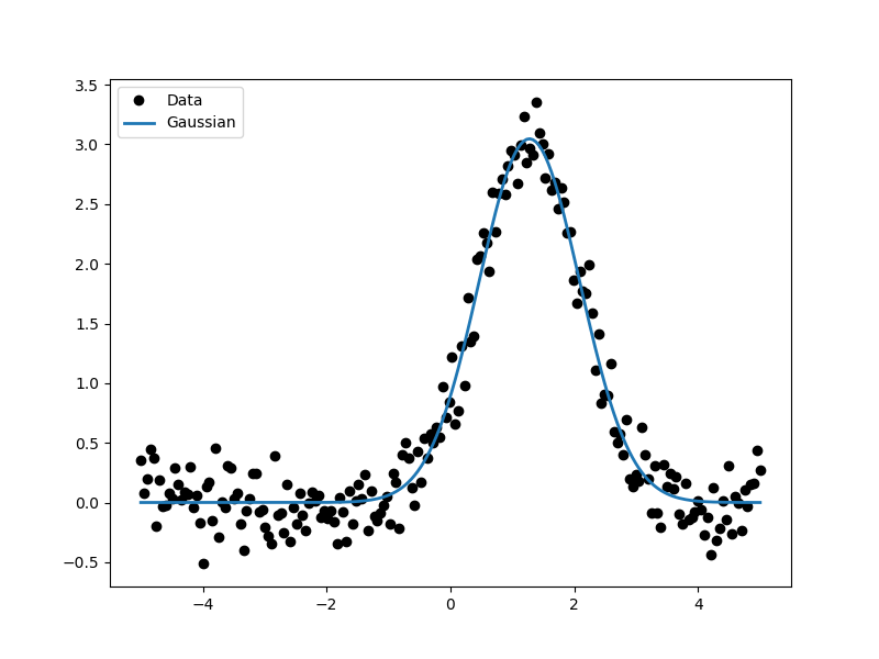
As the model can be evaluated directly, this plot can also be created manually:
>>> plt.plot(d.x, d.y, 'ko', label='Data')
>>> plt.plot(d.x, g(d.x), linewidth=2, label='Gaussian')
>>> plt.legend(loc=2);
Extract the parameter values
The fit results include a large number of attributes, many of which
are not relevant here (as the fit was done with no error values).
The following relation is used to convert from the full-width
half-maximum value, used by the Gauss1D
model, to the Gaussian sigma value used to create the data:
\(\rm{FWHM} = 2 \sqrt{2ln(2)} \sigma\):
>>> print(gres)
datasets       = None
itermethodname = none
methodname     = levmar
statname       = leastsq
succeeded      = True
parnames       = ('gauss1d.fwhm', 'gauss1d.pos', 'gauss1d.ampl')
parvals        = (1.915724111406394, 1.2743015983545247, 3.0470560360944017)
statval        = 8.069746329529591
istatval       = 180.71034547759984
dstatval       = 172.64059914807027
numpoints      = 200
dof            = 197
qval           = None
rstat          = None
message        = successful termination
nfev           = 30
>>> conv = 2 * np.sqrt(2 * np.log(2))
>>> ans = dict(zip(gres.parnames, gres.parvals))
>>> print("Position = {:.2f}  truth= {:.2f}".format(ans['gauss1d.pos'], pos_true))
Position = 1.27  truth= 1.30
>>> print("Amplitude= {:.2f}  truth= {:.2f}".format(ans['gauss1d.ampl'], ampl_true))
Amplitude= 3.05  truth= 3.00
>>> print("Sigma    = {:.2f}  truth= {:.2f}".format(ans['gauss1d.fwhm']/conv, sigma_true))
Sigma    = 0.81  truth= 0.80
The model, and its parameter values, can also be queried directly, as they have been changed by the fit:
>>> print(g)
gauss1d
   Param        Type          Value          Min          Max      Units
   -----        ----          -----          ---          ---      -----
   gauss1d.fwhm thawed      1.91572  1.17549e-38  3.40282e+38
   gauss1d.pos  thawed       1.2743 -3.40282e+38  3.40282e+38
   gauss1d.ampl thawed      3.04706 -3.40282e+38  3.40282e+38
>>> print(g.pos)
val         = 1.2743015983545247
min         = -3.4028234663852886e+38
max         = 3.4028234663852886e+38
units       =
frozen      = False
link        = None
default_val = 0.0
default_min = -3.4028234663852886e+38
default_max = 3.4028234663852886e+38
Including errors
For this example, the error on each bin is assumed to be the same, and equal to the true error:
>>> dy = np.ones(x.size) * err_true
>>> de = Data1D('with-errors', x, y, staterror=dy)
>>> print(de)
name      = with-errors
x         = Float64[200]
y         = Float64[200]
staterror = Float64[200]
syserror  = None
The statistic is changed from least squares to
chi-square (Chi2), to take advantage
of this extra knowledge (i.e. the Chi-square statistic includes
the error value per bin when calculating the statistic value):
>>> from sherpa.stats import Chi2
>>> ustat = Chi2()
>>> ge = Gauss1D('gerr')
>>> gefit = Fit(de, ge, stat=ustat, method=opt)
>>> geres = gefit.fit()
>>> print(geres.format())
Method                = levmar
Statistic             = chi2
Initial fit statistic = 4517.76
Final fit statistic   = 201.744 at function evaluation 30
Data points           = 200
Degrees of freedom    = 197
Probability [Q-value] = 0.393342
Reduced statistic     = 1.02408
Change in statistic   = 4316.01
   gerr.fwhm      1.91572      +/- 0.0331963
   gerr.pos       1.2743       +/- 0.0140972
   gerr.ampl      3.04706      +/- 0.0457235
>>> if not geres.succeeded: print(geres.message)
Since the error value is independent of bin, then the fit results
should be the same here (that is, the parameters in g are the
same as ge):
>>> print(g)
gauss1d
   Param        Type          Value          Min          Max      Units
   -----        ----          -----          ---          ---      -----
   gauss1d.fwhm thawed      1.91572  1.17549e-38  3.40282e+38
   gauss1d.pos  thawed       1.2743 -3.40282e+38  3.40282e+38
   gauss1d.ampl thawed      3.04706 -3.40282e+38  3.40282e+38
>>> print(ge)
gerr
   Param        Type          Value          Min          Max      Units
   -----        ----          -----          ---          ---      -----
   gerr.fwhm    thawed      1.91572  1.17549e-38  3.40282e+38
   gerr.pos     thawed       1.2743 -3.40282e+38  3.40282e+38
   gerr.ampl    thawed      3.04706 -3.40282e+38  3.40282e+38
The difference is that more of the fields
in the result structure are populated: in particular the
rstat and
qval fields, which give the
reduced statistic and the probability of obtaining this statistic value
respectively.:
>>> print(geres)
datasets       = None
itermethodname = none
methodname     = levmar
statname       = chi2
succeeded      = True
parnames       = ('gerr.fwhm', 'gerr.pos', 'gerr.ampl')
parvals        = (1.9157241114064163, 1.2743015983545292, 3.047056036094392)
statval        = 201.74365823823976
istatval       = 4517.758636940002
dstatval       = 4316.014978701763
numpoints      = 200
dof            = 197
qval           = 0.3933424667915623
rstat          = 1.0240794834428415
message        = successful termination
nfev           = 30
Error analysis
The default error estimation routine is
Covariance, which will be replaced by
Confidence for this example:
>>> from sherpa.estmethods import Confidence
>>> gefit.estmethod = Confidence()
>>> print(gefit.estmethod)
name         = confidence
sigma        = 1
eps          = 0.01
maxiters     = 200
soft_limits  = False
remin        = 0.01
fast         = False
parallel     = True
numcores     = 4
maxfits      = 5
max_rstat    = 3
tol          = 0.2
verbose      = False
openinterval = False
Running the error analysis can take time, for particularly complex
models. The default behavior is to use all the available CPU cores
on the machine, but this can be changed with the numcores
attribute. Note that a message is displayed to the screen when each
bound is calculated, to indicate progress:
>>> errors = gefit.est_errors()
gerr.fwhm lower bound:      -0.0326327
gerr.fwhm upper bound:      0.0332578
gerr.pos lower bound:       -0.0140981
gerr.pos upper bound:       0.0140981
gerr.ampl lower bound:      -0.0456119
gerr.ampl upper bound:      0.0456119
The results can be displayed:
>>> print(errors.format())
Confidence Method     = confidence
Iterative Fit Method  = None
Fitting Method        = levmar
Statistic             = chi2
confidence 1-sigma (68.2689%) bounds:
   Param            Best-Fit  Lower Bound  Upper Bound
   -----            --------  -----------  -----------
   gerr.fwhm         1.91572   -0.0326327    0.0332578
   gerr.pos           1.2743   -0.0140981    0.0140981
   gerr.ampl         3.04706   -0.0456119    0.0456119
The ErrorEstResults instance returned by
est_errors() contains the parameter
values and limits:
>>> print(errors)
datasets    = None
methodname  = confidence
iterfitname = none
fitname     = levmar
statname    = chi2
sigma       = 1
percent     = 68.26894921370858
parnames    = ('gerr.fwhm', 'gerr.pos', 'gerr.ampl')
parvals     = (1.9157241114064163, 1.2743015983545292, 3.047056036094392)
parmins     = (-0.0326327431233302, -0.014098074065578947, -0.045611913713536456)
parmaxes    = (0.033257800216357714, 0.014098074065578947, 0.045611913713536456)
nfits       = 29
The data can be accessed, e.g. to create a dictionary where the keys are the parameter names and the values represent the parameter ranges:
>>> dvals = zip(errors.parnames, errors.parvals, errors.parmins,
... errors.parmaxes)
>>> pvals = {d[0]: {'val': d[1], 'min': d[2], 'max': d[3]}
             for d in dvals}
>>> pvals['gerr.pos']
{'min': -0.014098074065578947, 'max': 0.014098074065578947, 'val': 1.2743015983545292}
Screen output
The default behavior - when not using the default
Covariance method - is for
est_errors() to print out the parameter
bounds as it finds them, which can be useful in an interactive session
since the error analysis can be slow. This can be controlled using
the Sherpa logging interface.
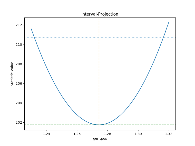
A single parameter
It is possible to investigate the error surface of a single
parameter using the
IntervalProjection class. The following shows
how the error surface changes with the position of the gaussian. The
prepare() method are given
the range over which to vary the parameter (the range is chosen to
be close to the three-sigma limit from the confidence analysis above,
ahd the dotted line is added to indicate the three-sigma
limit above the best-fit for a single parameter):
>>> from sherpa.plot import IntervalProjection
>>> iproj = IntervalProjection()
>>> iproj.prepare(min=1.23, max=1.32, nloop=41)
>>> iproj.calc(gefit, ge.pos)
This can take some time, depending on the complexity of the model and number of steps requested. The resulting data looks like:
>>> iproj.plot()
>>> plt.axhline(geres.statval + 9, linestyle='dotted');
The curve is stored in the
IntervalProjection object (in fact, these
values are created by the call to
calc() and so can be accesed without
needing to create the plot):
>>> print(iproj)
x     = [ 1.23  , 1.2323, 1.2345, 1.2368, 1.239 , 1.2412, 1.2435, 1.2457, 1.248 ,
  1.2503, 1.2525, 1.2548, 1.257 , 1.2592, 1.2615, 1.2637, 1.266 , 1.2683,
  1.2705, 1.2728, 1.275 , 1.2772, 1.2795, 1.2817, 1.284 , 1.2863, 1.2885,
  1.2908, 1.293 , 1.2953, 1.2975, 1.2997, 1.302 , 1.3043, 1.3065, 1.3088,
  1.311 , 1.3133, 1.3155, 1.3177, 1.32  ]
y     = [ 211.597 , 210.6231, 209.6997, 208.8267, 208.0044, 207.2325, 206.5113,
  205.8408, 205.2209, 204.6518, 204.1334, 203.6658, 203.249 , 202.883 ,
  202.5679, 202.3037, 202.0903, 201.9279, 201.8164, 201.7558, 201.7461,
  201.7874, 201.8796, 202.0228, 202.2169, 202.462 , 202.758 , 203.105 ,
  203.5028, 203.9516, 204.4513, 205.0018, 205.6032, 206.2555, 206.9585,
  207.7124, 208.5169, 209.3723, 210.2783, 211.235 , 212.2423]
min   = 1.23
max   = 1.32
nloop = 41
delv  = None
fac   = 1
log   = False
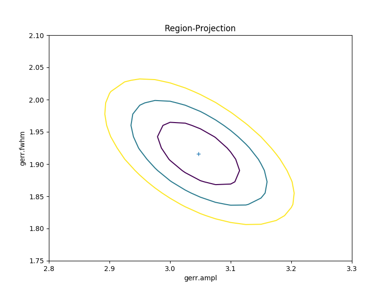
A contour plot of two parameters
The RegionProjection class supports
the comparison of two parameters. The contours indicate the one,
two, and three sigma contours.
>>> from sherpa.plot import RegionProjection
>>> rproj = RegionProjection()
>>> rproj.prepare(min=[2.8, 1.75], max=[3.3, 2.1], nloop=[21, 21])
>>> rproj.calc(gefit, ge.ampl, ge.fwhm)
As with the interval projection, this step can take time.
>>> rproj.contour()
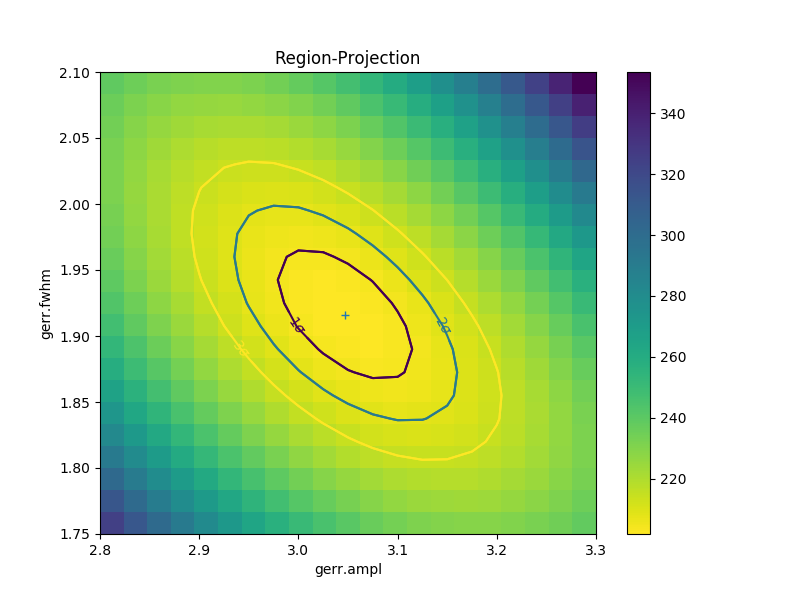
As with the single-parameter case, the statistic values for the grid are
stored in the RegionProjection object by the
calc() call,
and so can be accesed without needing to create the contour plot. Useful
fields include x0 and x1 (the two parameter values),
y (the statistic value), and levels (the values used for the
contours):
>>> lvls = rproj.levels
>>> print(lvls)
[ 204.03940717  207.92373254  213.57281632]
>>> nx, ny = rproj.nloop
>>> x0, x1, y = rproj.x0, rproj.x1, rproj.y
>>> x0.resize(ny, nx)
>>> x1.resize(ny, nx)
>>> y.resize(ny, nx)
>>> plt.imshow(y, origin='lower', cmap='viridis_r', aspect='auto',
...            extent=(x0.min(), x0.max(), x1.min(), x1.max()))
>>> plt.colorbar()
>>> plt.xlabel(rproj.xlabel)
>>> plt.ylabel(rproj.ylabel)
>>> cs = plt.contour(x0, x1, y, levels=lvls)
>>> lbls = [(v, r"${}\sigma$".format(i+1)) for i, v in enumerate(lvls)]
>>> plt.clabel(cs, lvls, fmt=dict(lbls));
Fitting two-dimensional data
Sherpa has support for two-dimensional data - that is data defined
on the independent axes x0 and x1. In the example below a
contiguous grid is used, that is the pixel size is constant, but
there is no requirement that this is the case.
>>> np.random.seed(0)
>>> x1, x0 = np.mgrid[:128, :128]
>>> y = 2 * x0**2 - 0.5 * x1**2 + 1.5 * x0 * x1 - 1
>>> y += np.random.normal(0, 0.1, y.shape) * 50000
Creating a data object
To support irregularly-gridded data, the multi-dimensional
data classes require
that the coordinate arrays and data values are one-dimensional.
For example, the following code creates a
Data2D object:
>>> from sherpa.data import Data2D
>>> x0axis = x0.ravel()
>>> x1axis = x1.ravel()
>>> yaxis = y.ravel()
>>> d2 = Data2D('img', x0axis, x1axis, yaxis, shape=(128, 128))
>>> print(d2)
name      = img
x0        = Int64[16384]
x1        = Int64[16384]
y         = Float64[16384]
shape     = (128, 128)
staterror = None
syserror  = None
Define the model
Creating the model is the same as the one-dimensional case; in this
case the Polynom2D class is used
to create a low-order polynomial:
>>> from sherpa.models.basic import Polynom2D
>>> p2 = Polynom2D('p2')
>>> print(p2)
p2
   Param        Type          Value          Min          Max      Units
   -----        ----          -----          ---          ---      -----
   p2.c         thawed            1 -3.40282e+38  3.40282e+38
   p2.cy1       thawed            0 -3.40282e+38  3.40282e+38
   p2.cy2       thawed            0 -3.40282e+38  3.40282e+38
   p2.cx1       thawed            0 -3.40282e+38  3.40282e+38
   p2.cx1y1     thawed            0 -3.40282e+38  3.40282e+38
   p2.cx1y2     thawed            0 -3.40282e+38  3.40282e+38
   p2.cx2       thawed            0 -3.40282e+38  3.40282e+38
   p2.cx2y1     thawed            0 -3.40282e+38  3.40282e+38
   p2.cx2y2     thawed            0 -3.40282e+38  3.40282e+38
Control the parameters being fit
To reduce the number of parameters being fit, the frozen attribute
can be set:
>>> for n in ['cx1', 'cy1', 'cx2y1', 'cx1y2', 'cx2y2']:
   ...:     getattr(p2, n).frozen = True
   ...:
>>> print(p2)
p2
   Param        Type          Value          Min          Max      Units
   -----        ----          -----          ---          ---      -----
   p2.c         thawed            1 -3.40282e+38  3.40282e+38
   p2.cy1       frozen            0 -3.40282e+38  3.40282e+38
   p2.cy2       thawed            0 -3.40282e+38  3.40282e+38
   p2.cx1       frozen            0 -3.40282e+38  3.40282e+38
   p2.cx1y1     thawed            0 -3.40282e+38  3.40282e+38
   p2.cx1y2     frozen            0 -3.40282e+38  3.40282e+38
   p2.cx2       thawed            0 -3.40282e+38  3.40282e+38
   p2.cx2y1     frozen            0 -3.40282e+38  3.40282e+38
   p2.cx2y2     frozen            0 -3.40282e+38  3.40282e+38
Fit the data
Fitting is no different (the same statistic and optimisation objects used earlier could have been re-used here):
>>> f2 = Fit(d2, p2, stat=LeastSq(), method=LevMar())
>>> res2 = f2.fit()
>>> if not res2.succeeded: print(res2.message)
>>> print(res2)
datasets       = None
itermethodname = none
methodname     = levmar
statname       = leastsq
succeeded      = True
parnames       = ('p2.c', 'p2.cy2', 'p2.cx1y1', 'p2.cx2')
parvals        = (-80.28947555488139, -0.48174521913599017, 1.5022711710872119, 1.9894112623568638)
statval        = 400658883390.66907
istatval       = 6571471882611.967
dstatval       = 6170812999221.298
numpoints      = 16384
dof            = 16380
qval           = None
rstat          = None
message        = successful termination
nfev           = 45
>>> print(p2)
p2
   Param        Type          Value          Min          Max      Units
   -----        ----          -----          ---          ---      -----
   p2.c         thawed     -80.2895 -3.40282e+38  3.40282e+38
   p2.cy1       frozen            0 -3.40282e+38  3.40282e+38
   p2.cy2       thawed    -0.481745 -3.40282e+38  3.40282e+38
   p2.cx1       frozen            0 -3.40282e+38  3.40282e+38
   p2.cx1y1     thawed      1.50227 -3.40282e+38  3.40282e+38
   p2.cx1y2     frozen            0 -3.40282e+38  3.40282e+38
   p2.cx2       thawed      1.98941 -3.40282e+38  3.40282e+38
   p2.cx2y1     frozen            0 -3.40282e+38  3.40282e+38
   p2.cx2y2     frozen            0 -3.40282e+38  3.40282e+38
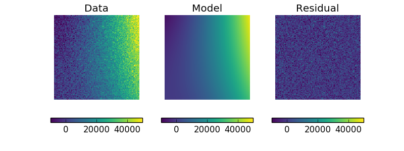
Display the model
The model can be visualized by evaluating it over a grid of points and then displaying it:
>>> m2 = p2(x0axis, x1axis).reshape(128, 128)
>>> def pimg(d, title):
...     plt.imshow(d, origin='lower', interpolation='nearest',
...                vmin=-1e4, vmax=5e4, cmap='viridis')
...     plt.axis('off')
...     plt.colorbar(orientation='horizontal',
...                  ticks=[0, 20000, 40000])
...     plt.title(title)
...
>>> plt.figure(figsize=(8, 3))
>>> plt.subplot(1, 3, 1);
>>> pimg(y, "Data")
>>> plt.subplot(1, 3, 2)
>>> pimg(m2, "Model")
>>> plt.subplot(1, 3, 3)
>>> pimg(y - m2, "Residual")
Note
The sherpa.image model provides support for interactive
image visualization, but this only works if the
DS9 image viewer is installed.
For the examples in this document, matplotlib plots will be
created to view the data directly.
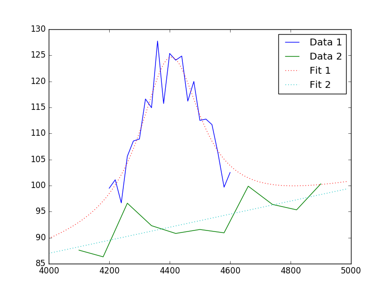
Simultaneous fits
Sherpa allows multiple data sets to be fit at the same time, although there is only really a benefit if there is some model component or value that is shared between the data sets). In this example we have a dataset containing a lorentzian signal with a background component, and another with just the background component. Fitting both together can improve the constraints on the parameter values.
First we start by simulating the data, where the
Polynom1D
class is used to model the background as a straight line, and
Lorentz1D
for the signal:
>>> from sherpa.models import Polynom1D
>>> from sherpa.astro.models import Lorentz1D
>>> tpoly = Polynom1D()
>>> tlor = Lorentz1D()
>>> tpoly.c0 = 50
>>> tpoly.c1 = 1e-2
>>> tlor.pos = 4400
>>> tlor.fwhm = 200
>>> tlor.ampl = 1e4
>>> x1 = np.linspace(4200, 4600, 21)
>>> y1 = tlor(x1) + tpoly(x1) + np.random.normal(scale=5, size=x1.size)
>>> x2 = np.linspace(4100, 4900, 11)
>>> y2 = tpoly(x2) + np.random.normal(scale=5, size=x2.size)
>>> print("x1 size {}  x2 size {}".format(x1.size, x2.size))
x1 size 21  x2 size 11
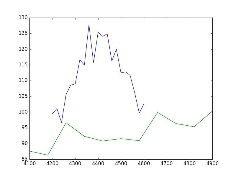
There is no requirement that the data sets have a common grid, as can be seen in a raw view of the data:
>>> plt.plot(x1, y1)
>>> plt.plot(x2, y2)
The fits are set up as before; a data object is needed for each data set, and model instances are created:
>>> d1 = Data1D('a', x1, y1)
>>> d2 = Data1D('b', x2, y2)
>>> fpoly, flor = Polynom1D(), Lorentz1D()
>>> fpoly.c1.thaw()
>>> flor.pos = 4500
To help the fit, we use a simple algorithm to estimate the starting point for the source amplitude, by evaluating the model on the data grid and calculating the change in the amplitude needed to make it match the data:
>>> flor.ampl = y1.sum() / flor(x1).sum()
For simultaneous fits the same optimisation and statistic needs to be used for each fit (this is an area we are looking to improve):
>>> from sherpa.optmethods import NelderMead
>>> stat, opt = LeastSq(), NelderMead()
Set up the fits to the individual data sets:
>>> f1 = Fit(d1, fpoly + flor, stat, opt)
>>> f2 = Fit(d2, fpoly, stat, opt)
and a simultaneous (i.e. to both data sets) fit:
>>> from sherpa.data import DataSimulFit
>>> from sherpa.models import SimulFitModel
>>> sdata = DataSimulFit('all', (d1, d2))
>>> smodel = SimulFitModel('all', (fpoly + flor, fpoly))
>>> sfit = Fit(sdata, smodel, stat, opt)
Note that there is a simulfit() method that
can be used to fit using multiple sherpa.fit.Fit objects,
which wraps the above (using individual fit objects allows some
of the data to be fit first, which may help reduce the parameter
space needed to be searched):
>>> res = sfit.fit()
>>> print(res)
datasets       = None
itermethodname = none
methodname     = neldermead
statname       = leastsq
succeeded      = True
parnames       = ('polynom1d.c0', 'polynom1d.c1', 'lorentz1d.fwhm', 'lorentz1d.pos', 'lorentz1d.ampl')
parvals        = (36.829217311393585, 0.012540257025027028, 249.55651534213359, 4402.7031194359088, 12793.559398547319)
statval        = 329.6525419378109
istatval       = 3813284.1822045334
dstatval       = 3812954.52966
numpoints      = 32
dof            = 27
qval           = None
rstat          = None
message        = Optimization terminated successfully
nfev           = 1152
The values of the numpoints and dof fields show that both datasets
have been used in the fit.
The data can then be viewed (in this case a separate grid is used, but the data objects could be used to define the grid):
>>> plt.plot(x1, y1, label='Data 1')
>>> plt.plot(x2, y2, label='Data 2')
>>> x = np.arange(4000, 5000, 10)
>>> plt.plot(x, (fpoly + flor)(x), linestyle='dotted', label='Fit 1')
>>> plt.plot(x, fpoly(x), linestyle='dotted', label='Fit 2')
>>> plt.legend();
How do you do error analysis? Well, can call sfit.est_errors(), but
that will fail with the current statistic (LeastSq), so need to
change it. The error is 5, per bin, which has to be set up:
>>> print(sfit.calc_stat_info())
name      =
ids       = None
bkg_ids   = None
statname  = leastsq
statval   = 329.6525419378109
numpoints = 32
dof       = 27
qval      = None
rstat     = None
>>> d1.staterror = np.ones(x1.size) * 5
>>> d2.staterror = np.ones(x2.size) * 5
>>> sfit.stat = Chi2()
>>> check = sfit.fit()
How much did the fit change?:
>>> check.dstatval
0.0
Note that since the error on each bin is the same value, the best-fit
value is not going to be different to the LeastSq result (so dstatval
should be 0):
>>> print(sfit.calc_stat_info())
name      =
ids       = None
bkg_ids   = None
statname  = chi2
statval   = 13.186101677512438
numpoints = 32
dof       = 27
qval      = 0.988009259609
rstat     = 0.48837413620416437
>>> sres = sfit.est_errors()
>>> print(sres)
datasets    = None
methodname  = covariance
iterfitname = none
fitname     = neldermead
statname    = chi2
sigma       = 1
percent     = 68.2689492137
parnames    = ('polynom1d.c0', 'polynom1d.c1', 'lorentz1d.fwhm', 'lorentz1d.pos', 'lorentz1d.ampl')
parvals     = (36.829217311393585, 0.012540257025027028, 249.55651534213359, 4402.7031194359088, 12793.559398547319)
parmins     = (-4.9568824809960628, -0.0011007470586726147, -6.6079122387075824, -2.0094070026087474, -337.50275154547768)
parmaxes    = (4.9568824809960628, 0.0011007470586726147, 6.6079122387075824, 2.0094070026087474, 337.50275154547768)
nfits       = 0
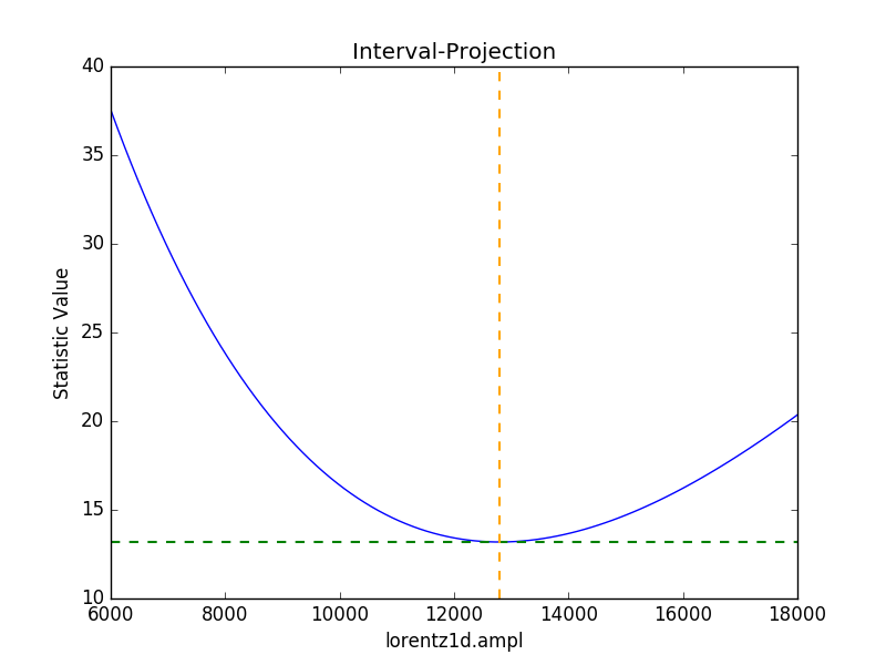
Error estimates on a single parameter are as above:
>>> iproj = IntervalProjection()
>>> iproj.prepare(min=6000, max=18000, nloop=101)
>>> iproj.calc(sfit, flor.ampl)
>>> iproj.plot()