Simulating data

A simple case

Simulating a data set normally involves:

evaluate the model

add in noise

This may need to be repeated several times for complex models, such as when different components have different noise models or the noise needs to be added before evaluation by a component.

The model evaluation would be performed using the techniques described in this section, and then the noise term can be handled with sherpa.utils.poisson_noise() or routines from NumPy or SciPy to evaluate noise, such as numpy.random.standard_normal.

>>> import numpy as np
>>> from sherpa.models.basic import Polynom1D

>>> np.random.seed(235)

>>> x = np.arange(10, 100, 12)
>>> mdl = Polynom1D('mdl')
>>> mdl.offset = 35
>>> mdl.c1 = 0.5
>>> mdl.c2 = 0.12

>>> ymdl = mdl(x)

>>> from sherpa.utils import poisson_noise
>>> ypoisson = poisson_noise(ymdl)

>>> from numpy.random import standard_normal, normal
>>> yconst = ymdl + standard_normal(ymdl.shape) * 10
>>> ydata = ymdl + normal(scale=np.sqrt(ymdl))

X-ray data (`DataPHA`)

In principle, the same steps apply when simulating PHA data (DataPHA objects), however, the mechanics are a little more complicated because we need to account for the instrumental response (ARF and RMF) and possibly also the background, which may contribute to the source spectrum that we want to simulate. Readers not interested in X-ray data analysis may want to skip this section.

Sherpa offers a dedicated function sherpa.astro.fake.fake_pha() for simulations of PHA data. A DataPHA object needs to be set up with the responses for the source and an exposure time. So, we first create a DataPHA object with the correct exposure time, but we can leave the settings for channel and counts empty, because these will be filled in by the simulation:

>>> from sherpa.astro.data import DataPHA
>>> from sherpa.astro.io import read_arf, read_rmf, read_pha
>>> data = DataPHA(name='any', channel=None, counts=None, exposure=10000.)
>>> data.set_arf(read_arf('9774.arf'))
>>> data.set_rmf(read_rmf('9774.rmf'))

Alternatively, one could read in a PHA file (data = read_pha('9774_bg.pi')). In this case, the response and backgrounds will be automatically loaded, if the relevant header keywords are set. Also, the exposure time, background scaling etc. will be taken from the header of the file. When new data is simulated later, the counts in data will be overwritten, but all other information stays the same.

Next, we set up a model. In this case, we start with a powerlaw source where the slope and normalization of that powerlaw are already known, e.g. from the literature. We then add a weak emission line. Our simulation will show us if this emission line would be detectable in a real observation:

>>> from sherpa.models.basic import PowLaw1D, Gauss1D
>>> pl = PowLaw1D()
>>> line = Gauss1D()
>>> pl.gamma = 1.8
>>> pl.ampl = 2e-05
>>> line.pos = 6.7
>>> line.ampl = .0003
>>> line.fwhm = .1
>>> srcmdl = pl + line

The simplest case: Simulate the source spectrum only

With this model, it is now easy to run the simulation, which will calculate the expected number of counts in each spectral channel (where the number and width of the channels is given by the responses) and then draw from a Poisson distribution with this expected number. Thus, the simulated number of counts in each channel is always an integer and includes Poisson noise - running fake_pha() twice with identical settings will give slightly different answers. With default settings, the input model is convolved with the RMF and multiplied by the ARF, and properly scaled for the exposure time.

>>> from sherpa.astro.fake import fake_pha
>>> fake_pha(data, srcmdl)

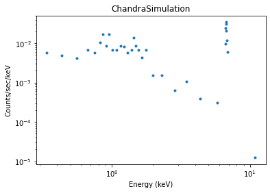
We bin the counts into bins of at least 5 counts per bin and display an image of the simulated spectrum (see X-ray data (DataPHA) for details):

>>> data.set_analysis('energy')
>>> data.notice(0.3, 8)
>>> data.group_counts(5)
>>> from sherpa.plot import DataPlot
>>> dplot = DataPlot()
>>> dplot.prepare(data)
>>> dplot.plot(xlog=True, ylog=True)

Sometimes, more than one response is needed, e.g. in Chandra LETG/HRC-S different orders of the grating overlap on the detector, so they all contribute to the observed source spectrum. fake_pha() works if one or more responses are set for the input DataPHA object.

It is also possible that the input model already includes the appropriate responses and scalings. In this case, is_source=False can be set to indicate to sherpa that the model is not a naked source model, but includes all required instrumental effects. In this way, fake_pha() can be used with arbitrarily complex models which may include such components as the instrumental backgound (which should not be folded through the ARF) or arbitary other components:

>>> fake_pha(data, model=inst_bkg + my_arf(my_rmf(srcmodel)), is_source=False)

Adding background

Weak spectral features can be hidden in a large (instrumental or astrophysical) background, thus it can be important to include background in the simulation.

Sample background from a PHA file

One way to include background is to sample it from a DataPHA object. To do so, a background need to be loaded into the dataset before running the simluation and, if not done before, the scale of the background scaling has to be set:

>>> data.set_background(read_pha('9774_bg.pi'))
>>> data.backscal = 9.6e-06
>>> fake_pha(data, srcmdl, add_bkgs=True)

The fake_pha function simulates the source spectrum as above, but then it samples from the background PHA. For each bin, it treats the background count number as the expected value and performs a Poisson draw. The background drawn from the Poisson distribution is than added to the simulated source spectrum (the sum of two Poisson distributions is a Poisson distribution again). This works best if the background is well exposed and has a large number or counts.

Why do we need to set the add_bkgs=True argument and do not simply use all available backgrounds? The reason for that is it is often useful to read in a file with data = read_pha('9774.pi'), which might automatically read in the background as well. Using the add_bkgs to switch the background on or off in the simulation makes it easy to compare the same simulation with and without a background.

Background models

When the number of counts in the background is low, the above procedure amplifies the noise. The experimental background already contains noise just from Poisson statistics. Using the observed count numbers as background value and then performing a Poisson draw on them again gives a higher level of noise than a real observation would have. To avoid this problem, a background model may be used instead:

>>> from sherpa.models.basic import Const1D
>>> bkgmdl = Const1D('bmdl')
>>> bkgmdl.c0 = 2
>>> fake_pha(data, mdl, add_bkgs=True, bkg_models={'1': bkgmdl})

The keys in the bkg_models dictionary are the identifiers of the backgrounds. Above, we loaded a background with the default identifyer (which is 1).

More than one background

If more than one background is set up, then the expected backgrounds will be averaged before the Poisson draw. For some backgrounds that expected value might be the value of the counts in a PHA file, while for others the expected value might be calculated from a model.

Reference/API

Simulate PHA datasets

The fake_pha routine is used to create simulated sherpa.astro.data.DataPHA data objects.

Functions

fake_pha(data, model[, is_source, ...])

Simulate a PHA data set from a model.