Help! My fit is too slow or doesn’t converge at all
There is no one recipe that will solve every fitting problem, but there are some common themes that can make the fitting process more efficient and robust. Many of the strategies below effect both the speed and the robustness of the fit, so they are listed together starting with what is usually the easiest and most effective to set up.
For illustration, we will use a simple example of a noisy dataset with some feature in it. This could represent e.g. a spectrum with an emission line. We pick this example because it is easy to see what is going on, but the same principles hold for more complex datasets, too. Here is code that generates data for this example:
>>> import numpy as np
>>>
>>> from sherpa.data import Data1D
>>> from sherpa.models import Const1D, Gauss1D, NormGauss1D
>>> from sherpa.stats import Chi2, Chi2Gehrels
>>> from sherpa.optmethods import LevMar, MonCar
>>> from sherpa.fit import Fit
>>> true_model = Const1D('continuum') + Gauss1D('line_1')
>>> true_model['continuum'].c0 = 1.
>>> true_model['line_1'].ampl = 0.5
>>> true_model['line_1'].pos = 652.28
>>> true_model['line_1'].fwhm = 1.23
>>>
>>> wave = np.arange(645, 660, 0.1)
>>>
>>> rng = np.random.default_rng(42)  # fixed seed for reproducibility
>>> spectrum = Data1D('spectal order 34', x=wave,
...                   y=true_model(wave) + rng.normal(0, 0.1, len(wave)),
...                   staterror=0.1 * np.ones(len(wave)))
Start close to the solution
So, let’s go ahead and fit this data with a model and plot the result (it is always a good idea to visually look at a result):
>>> model = Const1D('continuum') + Gauss1D('Halpha')
>>> fit = Fit(data=spectrum, model=model, stat=Chi2(), method=LevMar())
>>> result = fit.fit()
>>> from sherpa.plot import DataPlot, ModelPlot
>>> dplot = DataPlot()
>>> dplot.prepare(spectrum)
>>> dplot.xlabel = 'Wavelength (nm)'
>>> dplot.ylabel = 'flux (normalized)'
>>> mplot = ModelPlot()
>>> mplot.prepare(fit.data, fit.model)
>>> dplot.plot()
>>> mplot.overplot()
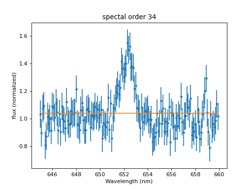
The continuum looks reasonable, but where is the Gaussian? We can see what happened by looking at the model values after the fit:
>>> print(model)
continuum + Halpha
   Param        Type          Value          Min          Max      Units
   -----        ----          -----          ---          ---      -----
   continuum.c0 thawed      1.03858 -3.40282e+38  3.40282e+38
   Halpha.fwhm  thawed           10  1.17549e-38  3.40282e+38
   Halpha.pos   thawed            0 -3.40282e+38  3.40282e+38
   Halpha.ampl  thawed            1 -3.40282e+38  3.40282e+38
The position of the Gaussian is at 0, where it started. Most models default start values around 0 or 1, so that they work well for normalized data. However, here we have no data below 645 at all, so when the optimizer tries out a few values around 0 for the position of the Gaussian, there is no difference in the fit statistic. Thus, it is always a good idea to set the starting values of the model parameters to some number close to the expected solution, or at least in the range of the data. If we do that, the fit immediately improves:
>>> model['Halpha'].pos = 652
>>> result = fit.fit()
>>> mplot.prepare(fit.data, fit.model)
>>> dplot.plot()
>>> mplot.overplot()
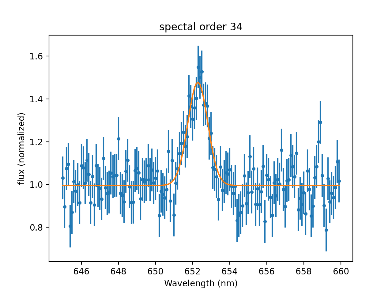

Of course, we want to perform the fit to find the best values because we do not know them yet. Still, in many cases, we can make good guesses about the starting values. For example, we may know that we are looking for a specific emission line that may be shifted in wavelength due to the red-shift of a star of galaxy. Even if we do not know the exact position, starting from the rest-wavelength might be close enough. Similarly, if we want to determine the distribution of the weight of some product we manufacture, we may know that the machine was set to package 100 g, so we can start from that value.
For simple models, the guess method can help with setting
starting values:
>>> # First, reset the model to the original values after the fit above
>>> model.reset()
>>> model['Halpha'].pos = 0
>>> print(model)
continuum + Halpha
   Param        Type          Value          Min          Max      Units
   -----        ----          -----          ---          ---      -----
   continuum.c0 thawed            1 -3.40282e+38  3.40282e+38
   Halpha.fwhm  thawed           10  1.17549e-38  3.40282e+38
   Halpha.pos   thawed            0 -3.40282e+38  3.40282e+38
   Halpha.ampl  thawed            1 -3.40282e+38  3.40282e+38
>>> fit.guess()
>>> print(model)
continuum + Halpha
   Param        Type          Value          Min          Max      Units
   -----        ----          -----          ---          ---      -----
   continuum.c0 thawed      1.16807   0.00786795      154.935
   Halpha.fwhm  thawed         7.45      0.00745         7450
   Halpha.pos   thawed        652.3          645        659.9
   Halpha.ampl  thawed      1.54935   0.00154935      1549.35
We can see that the guess method has set the position of the Gaussian to
the position of the maximum in the data and restricted the range for the position
to the range of the data. That is a reasonable guess, but not always correct, e.g.
we could have a really strong peak that is just outside the data range and that we
want to fit based on just a broad wing that we see inside the data range.
In other cases, the guess is probably looser than it has to be, e.g. the max for
the continuum is set way above the highest data point. The guess provides a good
starting point in many cases, but it is always a good idea to check the
numbers.
Set minimum and maximum values for parameters
Even when we set a starting value, sometimes the fit runs in the wrong
direction. In our example, we might start with model['Halpha'].pos = 648
and instead of converging to the right position, the optimizer might try smaller
and smaller values until it runs out of the data range. We can prevent that by
setting the minimum and maximum values for the parameters.
Even if we do not know the exact range, we usually can still restrict the order of magnitude based on what we know about the data. For example, we might know that the detector would be saturated above 50, and we know that we continuum-normalized our spectrum, so the continuum level should be close to 1. Since the total signal cannot fall below 0, that means that the lowest amplitude that is possible is about -1 (give or take a little, depending on how well the continuum normalization was done), so it would be safe the set the following limits:
>>> model['Halpha'].ampl.min = -2
>>> model['Halpha'].ampl.max = 50
Some optimizers attempt to explore the full parameters space (often called
“global optimizers”). If there are many parameters, this exploration is
necessarily sparse, e.g. putting just 10 points in each dimension
would require \(10^n\) points for n parameters. Thus, it is important that the
min and max values for the parameters are set to reasonable values.
For example, exploring the amplitude or position of a Gaussian in the default range
in ten evenly spaced steps
would use [-3.4e+38, -2.6e+38, -1.9e+38, -1.1e+38, -3.8e+37, 3.8e+37,
1.1e+38, 1.9e+38, 2.6e+38, 3.4e+38] - the closest number in that list is
37 magnitudes away from the best-fit. It is usually OK to allow the fit to
explore a slightly larger range than expected, but the default boundaries are
set to the maximum and minimum number that can be represented in a 32-bit
floating point number, which is far too wide for most use cases.
Reduce the number of parameters
Sometimes, we know the relation between two parameters, e.g. we have several features that have the same width or we know that one Gaussian is exactly twice a high as the other. In this case, we can link the parameters together to reduce the number of parameters that the optimizer has to explore. That will speed up the fit because the space to explore is smaller and typically also reduces the number of local minima where the optimizer might get stuck.
Use the model cache for speed-up
Except for the models that are expressed as a simple numerical function
(e.g. Const1D or Gauss1D),
the evaluation of the model is typically the most time-consuming part
of the fitting process. Thus, a fit can be sped up by evaluating the
model components fewer times. Models provided by Sherpa try to cache
the results of a model evaluation, so that the same calculation does
not have to be done a second time when the same parameters are used.
This happens more often than one might think, because many optimizers
change one parameter at a time. So, in our example, when the optimizer
changes continuum.c0, the Gaussian component will be repeatedly
evaluated at the same parameter values. See
Caching model evaluations for details on caching.
If multiple datasets with different grids are fit with the same model, the model will still be evaluated for every grid, so the size of the cache must be large enough to hold all the values, e.g. for fitting eight different datasets with the same model, the cache size should be at least 8 (the default for most models is 5):
>>> from sherpa.models import Erf
>>> erf = Erf('erf')
>>> erf.cache = 8
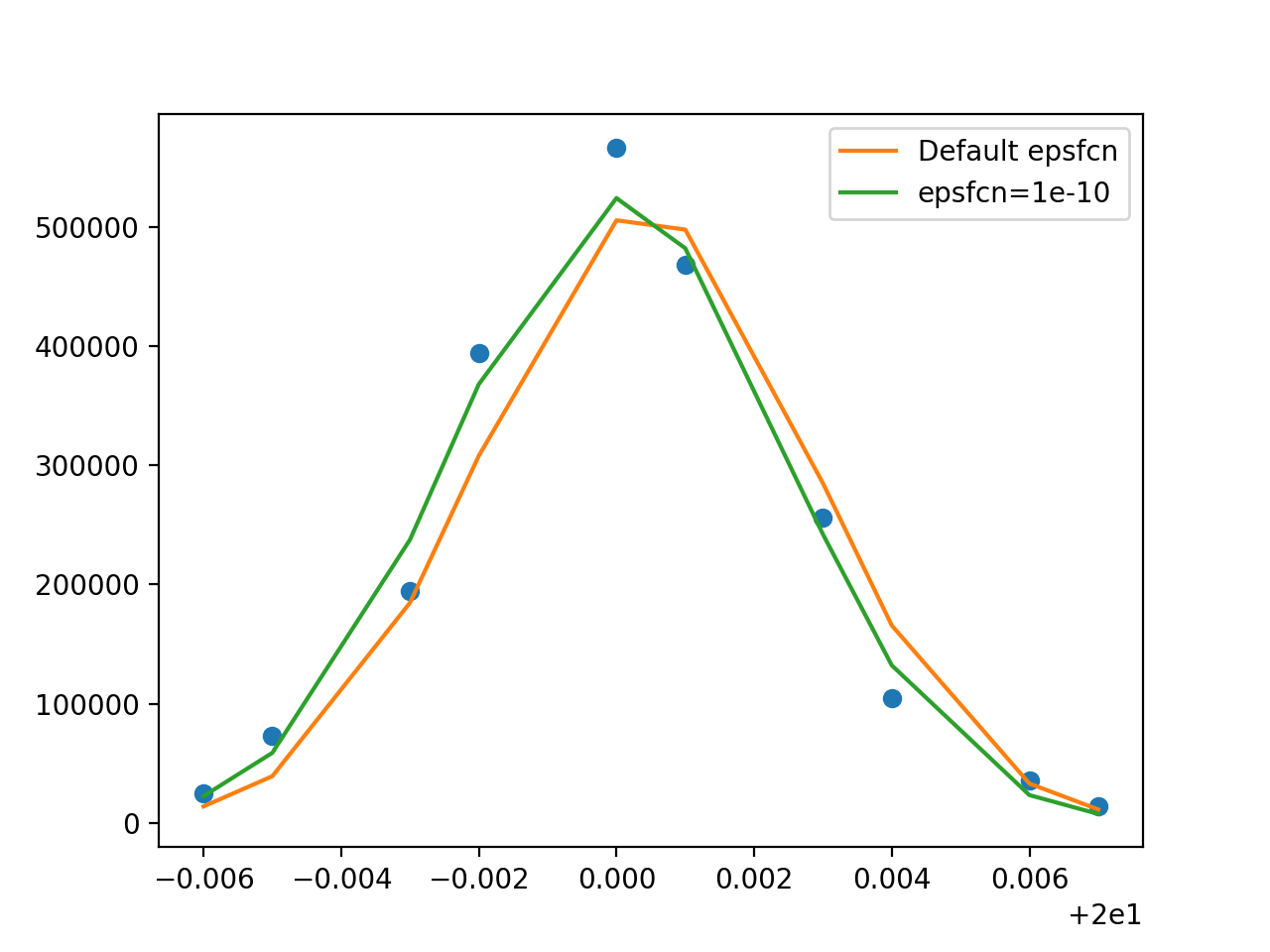
Increase the numerical precision
The default setting for the optimizers built into Sherpa is to stop further
iterations when the changes between steps are close to single precision
floating point precision because some models in the xspec
module are implemented in single precision FORTRAN and would never finish
if a higher precision was requested.
However, if your data or model has numbers of very different
scales, a small change in one parameter may not be detected in single
precision, leading to a bad fit. In this case, simply run the fit with a
higher precision using the epsfcn parameter of the optimizer:
>>> import matplotlib.pyplot as plt
>>> x = [20.007, 20.006, 20.004, 20.003, 20.001, 20., 19.998, 19.997, 19.995, 19.994]
>>> y = [13812, 35935, 104981, 256023, 468129, 566540, 393826, 194178, 73352, 25078]
>>> d = Data1D('linedata', x, y)
>>>
>>> howwide = NormGauss1D('gauss')
>>> howwide.fwhm = 0.01
>>> howwide.pos = 20.
>>> howwide.ampl = np.max(y) * 0.005
>>> linefit = Fit(d, howwide)
>>> result1 = linefit.fit()
>>>
>>> _ = plt.plot(d.x, d.y, 'o')
>>> _ = plt.plot(d.x, howwide(d.x), label='Default epsfcn')
>>>
>>> # Reset model to the same starting values
>>> howwide.reset()
>>> # Repeat the fit with a higher numerical precision
>>> linefit.method.config['epsfcn'] = 1e-10
>>> result2 = linefit.fit()
>>> _ = plt.plot(d.x, howwide(d.x), label='epsfcn=1e-10')
>>> _ = plt.legend()
>>> print(f"Fit 1 - final statistic: {result1.statval:5.0g} in {result1.nfev} steps")
Fit 1 - final statistic: 9e+04 in 53 steps
>>> print(f"Fit 2 - final statistic: {result2.statval:5.0g} in {result2.nfev} steps")
Fit 2 - final statistic: 3e+04 in 25 steps
Note how the fit with the default epsfcn parameter ends up to the right of the data,
while the fit with epsfcn=1e-10 is closer to the data. Neither result is perfect because the
data does not have a Gaussian shape, but at least the position for the second fit
is better, and the fit statistic is three times lower (it’s still so large that
we know we do not have a good fit, probably because we did not specify our
measurement errors in this example).
Also, in this particular case the fit with the better precision took only 25 steps,
while the first one took 53 steps, saving us about half the run time. That is
however not universal. Depending on the data and the model, a fit with a higher
precision may take longer or shorter.
Normalize the data
It is often convenient to work in the natural units of the data. In our example, we use the measured wavelength on the x-axis and the normalized flux on the y-axis. That way, we can read off the fitted position and width of the Gaussian directly. However, there is a second reason beyond numerical precision why that can make fitting difficult.
Since the optimizer does not know anything about the physics behind the data most optimizers start with the same step size in every direction. That can lead to problems if a step size of 1 in one direction is so small that is does not change the fit statistic (e.g. a change of the amplidude in the previous example), while a step size of 1 in another direction is so large that it immediately jumps our of the data range (e.g. a change of the position of the Gaussian in the previous example).
In that case, it might be a good idea to scale that data in some way so that all relevant scales are close to 1. For the previous dataset, one might try something similar to this:
>>> y_scale = np.mean(y)
>>> x_offset = np.mean(x)
>>> x_scale = np.std(x)
>>> d_scaled = Data1D('linedata_scaled',
...                   x = (x - x_offset) / x_scale,
...                   y = y / y_scale)
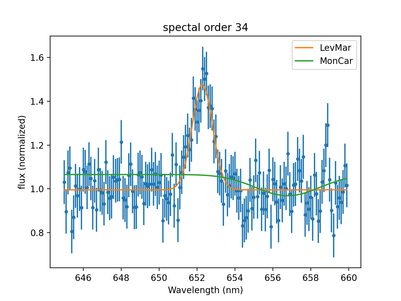
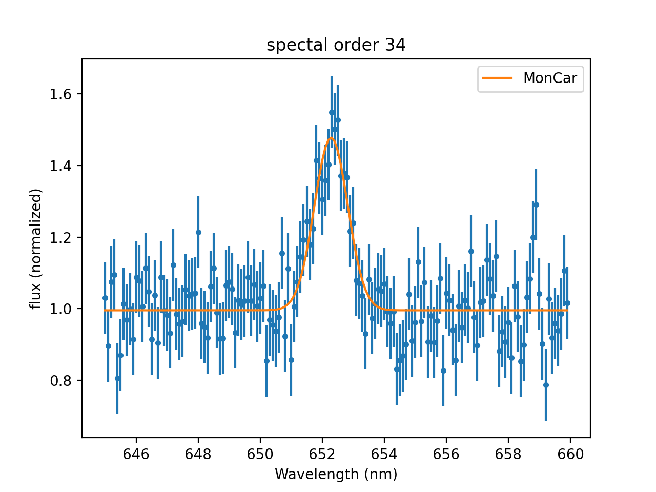
Try different optimizers
Sherpa provides different optimizers with different strengths and weaknesses. If one optimizer does not work well, try another one and you might get a different result. Here we go back to the dataset we used in the beginning and try a different optimizer:
>>> model.reset()
>>> model['Halpha'].ampl.min = -1e7
>>> model['Halpha'].pos = 650
>>> fit_result1 = fit.fit()
>>> mplot.prepare(fit.data, fit.model)
>>> dplot.plot()
>>> mplot.overplot(label='LevMar')
>>>
>>> model.reset()
>>> fit.method = MonCar()
>>> fit_result2 = fit.fit(record_steps=True)
>>> mplot.prepare(fit.data, fit.model)
>>> mplot.overplot(label='MonCar')

If the answers from different optimizers are similar, that is usually a good sign, though not a guarantee that the best fit has been found. If they are different, that deserves a closer look.
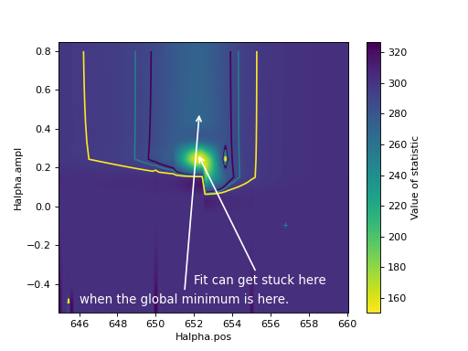
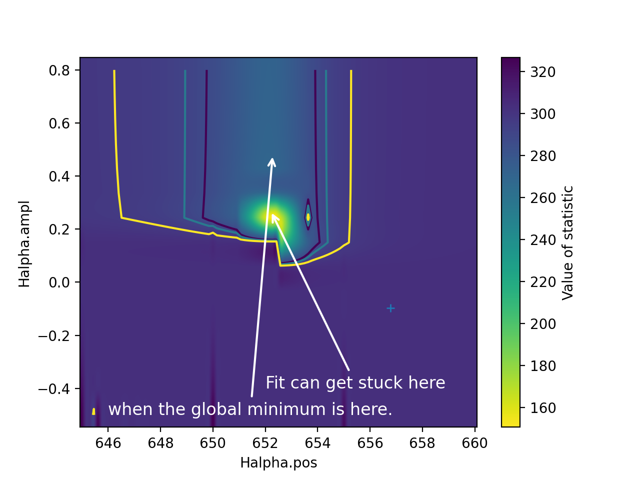
Look at the shape of the statistic function
Even in our simple example with four parameters, we cannot visualize the shape of the statistic function so see where the minimum is and it takes too long to calculate the statistic for every combination of parameters. However, we can look at a slice of just two parameters in the range we care about most and try to understand what is happening.
>>> import matplotlib.pyplot as plt
>>> from sherpa.plot import RegionProjection
>>> # We refit at every point, pick a fast method
>>> fit.method = LevMar()
>>> rproj = RegionProjection()
>>>
>>> rproj.prepare(min=(645, -.5), max=(660, .8), nloop=(100, 15))
>>> rproj.calc(fit, model['Halpha'].pos, model['Halpha'].ampl)
>>> xmin, xmax = rproj.x0.min(), rproj.x0.max()
>>> ymin, ymax = rproj.x1.min(), rproj.x1.max()
>>> nx, ny = rproj.nloop
>>> hx = 0.5 * (xmax - xmin) / (nx - 1)
>>> hy = 0.5 * (ymax - ymin) / (ny - 1)
>>> extent = (xmin - hx, xmax + hx, ymin - hy, ymax + hy)
>>> y = rproj.y.reshape((ny, nx))
>>> # The following commands return an object that is not used below.
>>> # To avoid extra output on the screen, we assign it to `_`
>>> _ = plt.imshow(y, origin='lower', extent=extent, aspect='auto', cmap='viridis_r',
...                interpolation='spline16')
>>> _ = plt.colorbar(label='Value of statistic')
>>> _ = plt.xlabel(rproj.xlabel)
>>> _ = plt.ylabel(rproj.ylabel)
>>> rproj.contour(overplot=True)
>>> _ = plt.annotate("Fit can get stuck here",
...                     xy=(652.2, 0.27),
... xytext=(652, -.4),
... arrowprops=dict(arrowstyle='->', lw=1.5, color='w'),
... fontsize=12, color='w')
>>> _ = plt.annotate("when the global minimum is here.", xy=fit_result1.parvals[2:],
... xytext=(646, -.5),
... arrowprops=dict(arrowstyle='->', lw=1.5, color='w'),
... fontsize=12, color='w')

The contours and the background image show the value of the statistic as a function of the two parameters.
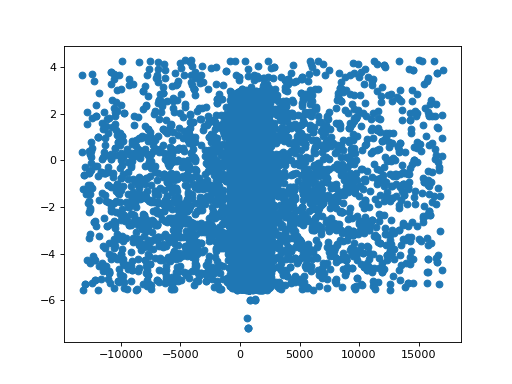
See the space explored by the optimizer
Similarly, we can visualize the space explored by the optimizer. Above,
we used the record_steps option for the MonCar optimizer, so all the values
that this optimizer tried are stored in the output and we can plot them
(or at least a subset that we can display in 2D or 3D):
>>> _ = plt.scatter(fit_result2.record_steps['Halpha.pos'],
...                 fit_result2.record_steps['Halpha.ampl'])
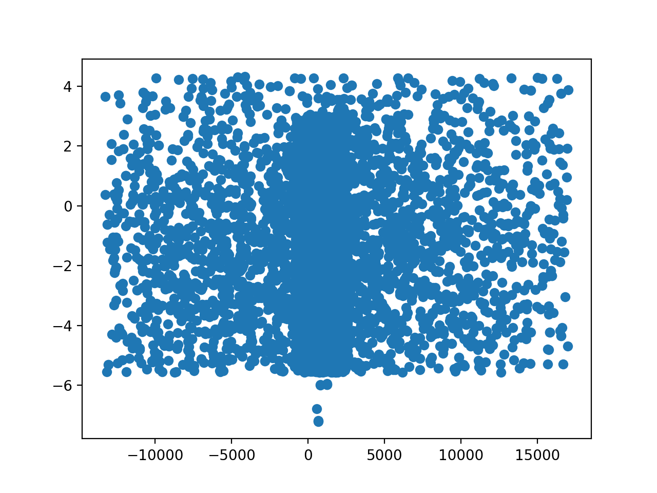

Woops! We forgot to Set minimum and maximum values for parameters and MonCar is a global optimizer, so it jumped way outside the data range. Let’s fix that and try again:
>>> model['Halpha'].pos.min = 645
>>> model['Halpha'].pos.max = 660
>>> model['Halpha'].ampl.min = -2
>>> model['Halpha'].ampl.max = 50
>>> model['Halpha'].fwhm.min = 0.1
>>> model['Halpha'].fwhm.max = 50
>>> model['continuum'].c0.min = 0
>>> model['continuum'].c0.max = 10
>>>
>>> fit.method = MonCar()
>>> fit.method.rng = rng
>>> fit_result3 = fit.fit(record_steps=True)
>>> _= plt.scatter(fit_result3.record_steps['Halpha.pos'],
...                fit_result3.record_steps['Halpha.ampl'])
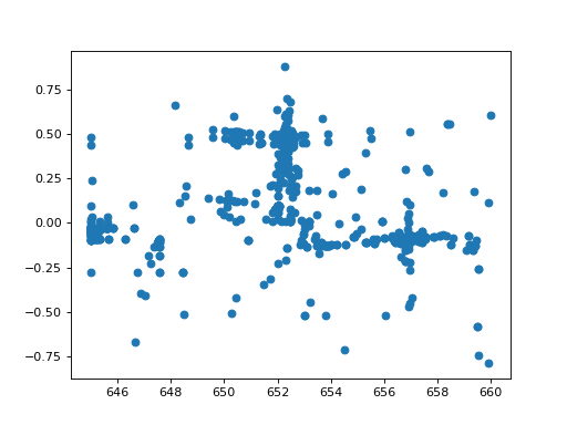
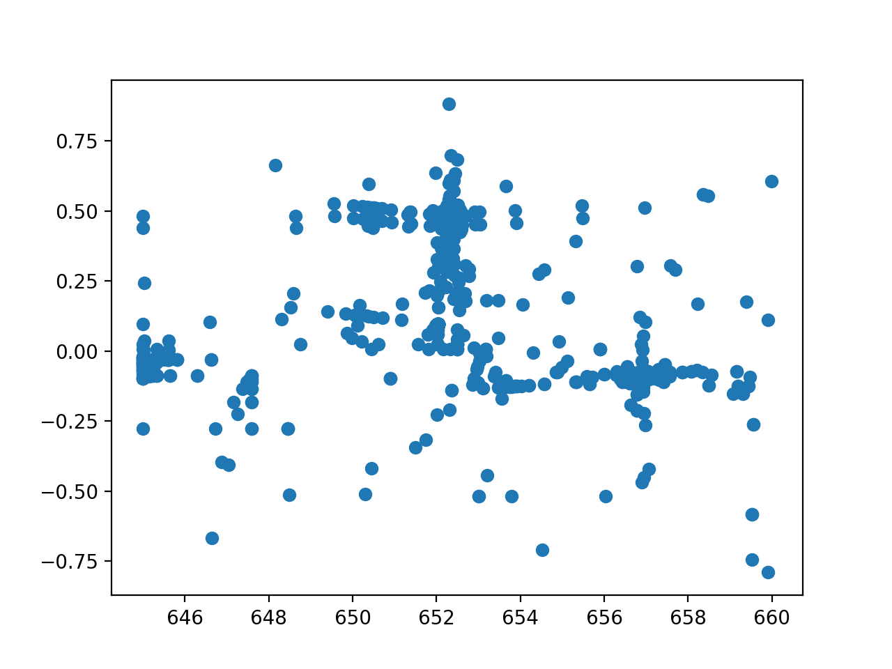

Now, we can see that the optimizer explored the range around the position where is started in great detail and gave us a good fit:
>>> dplot.plot()
>>> mplot.prepare(fit.data, fit.model)
>>> mplot.overplot(label='MonCar')
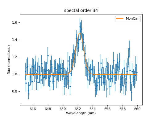

Adjust the parameters of the optimizer
If more control is needed, we can adjust the behavior of the optimizer.
All optimizers have specific parameters that control how they work,
e.g. that set the initial size of steps or the maximum number of iterations.
For MonCar we can make the search more robust
by making it more likely to jump in directions that do not improve the
fit statistic, which can allow the optimizer to escape local minima.
>>> fit.method.weighting_factor = 0.5
>>> fit.method.xprob = 0.5