Simultaneous fits
Sherpa uses the DataSimulFit and
SimulFitModel
classes to fit multiple datasets and models simultaneously.
This can be done explicitly, by combining individual data sets
and models into instances of these classes, or implicitly
with the simulfit() method.
It only makes sense to perform a simultaneous fit if there is some “link” between the various data sets or models, such as sharing one or more model components or linking model parameters.
Example
This example replicates fitting a few forbidden emission lines in an echelle spectrum where one line shows up in more than one order. The spectrum is noisy, so we want to use all the available data to constrain the fit. In reality, we would load the data from a file, but for the purpose of this example we will simulate two orders. One of them contains just the [Si II] line at 6716 Ang, while the other one contains both this line and the second member of the [Si II] doublet at 6731 Ang.
>>> import numpy as np
>>> from sherpa.models import Gauss1D
>>> wave_order26 = np.arange(6686, 6720, 1.1)
>>> wave_order27 = np.arange(6705, 6735, 1.2)
>>> rng = np.random.default_rng(seed=1234)
>>> # Make two components to simulate the lines
>>> line1 = Gauss1D('line1')
>>> line1.pos = 6716
>>> line1.fwhm = 2
>>> line1.ampl = 0.5
>>> line2 = Gauss1D('line2')
>>> line2.pos = 6731
>>> line2.fwhm = 2
>>> line2.ampl = 1
>>> # Flux is normalized to about 1, but not exactly right
>>> flux_order26 = rng.normal(0.98, 0.1, size=len(wave_order26))
>>> flux_order26 += line1(wave_order26)
>>> flux_order27 = rng.normal(1.11, 0.1, size=len(wave_order27))
>>> flux_order27 += line1(wave_order27) + line2(wave_order27)
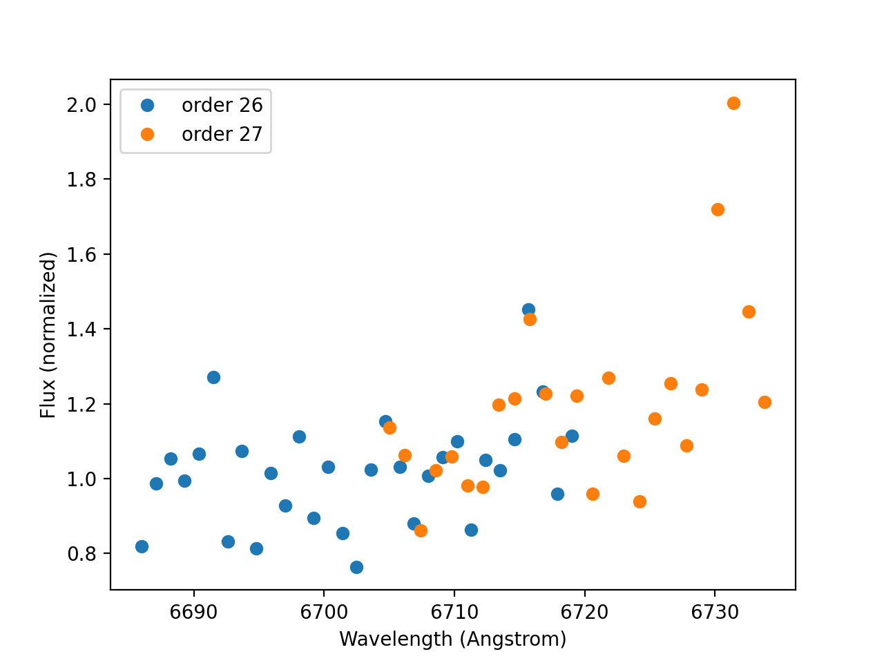
Let’s now do a quick plot of what we simulated. For real data, we would want to get an idea what it looks before fitting!
>>> from matplotlib import pyplot as plt
>>> _ = plt.plot(wave_order26, flux_order26, 'o', label='order 26')
>>> _ = plt.plot(wave_order27, flux_order27, 'o', label='order 27')
>>> _ = plt.xlabel('Wavelength (Angstrom)')
>>> _ = plt.ylabel('Flux (normalized)')
>>> _ = plt.legend()

So, we notice that there is a slight offset between the two orders. Let’s assume that we check our data reduction pipeline and find that this comes from some additional background in order 27 that looks constant over the order, so we decide to simply model that with a constant. We also know that we used a low-resolution grating, and thus the lines are not resolved and should have the same width, given how close they are in wavelength. We will link their FWHM parameters. We chose not to make an assumption about the ratio of the amplitudes of both lines, but, upon inspection of the plot, it seems that the wavelengths between the two orders are consistent (as they should be), so we can use the same model for the lines in both orders. Let’s set up the model we want to fit and set reasonable initial values for the parameters.
>>> from sherpa.models import Const1D, Gauss1D
>>> s_ii_6716 = Gauss1D('s_ii_6716')
>>> s_ii_6716.pos = 6716
>>> s_ii_6716.fwhm = 1.
>>> s_ii_6716.ampl = 1.
>>> s_ii_6731 = Gauss1D('s_ii_6731')
>>> s_ii_6731.pos = 6731.
>>> s_ii_6731.fwhm = s_ii_6716.fwhm
>>> s_ii_6731.ampl = 1.
>>> cont = Const1D('cont')
>>> extra_cont_order27 = Const1D('extra_cont_order27')
>>> model_26 = cont + s_ii_6716 + s_ii_6731
>>> model_27 = cont + extra_cont_order27 + s_ii_6716 + s_ii_6731
Now, we put the data into Sherpa’s data structures:
>>> from sherpa.data import Data1D
>>> flux_err_26 = 0.1 * np.ones_like(flux_order26)
>>> flux_err_27 = 0.1 * np.ones_like(flux_order27)
>>> data_26 = Data1D('order26', wave_order26, flux_order26, staterror=flux_err_26)
>>> data_27 = Data1D('order27', wave_order27, flux_order27, staterror=flux_err_27)
Finally, we can put it all together to make joint data, model, and fit objects to use for joint fitting and plot the result:
>>> from sherpa.data import DataSimulFit
>>> from sherpa.models import SimulFitModel
>>> from sherpa.stats import Chi2
>>> from sherpa.optmethods import LevMar
>>> from sherpa.fit import Fit
>>> data = DataSimulFit(name='both orders', datasets=(data_26, data_27))
>>> model = SimulFitModel(name='both', parts=(model_26, model_27))
>>> fit = Fit(data, model, method=LevMar(), stat=Chi2())
>>> result = fit.fit()
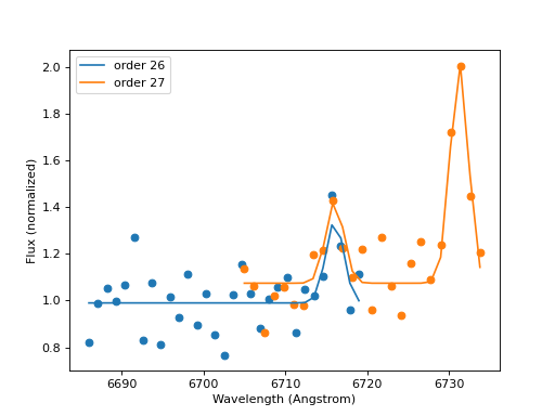
The fit results look good for both orders:
>>> _ = plt.plot(wave_order26, flux_order26, 'o')
>>> _ = plt.plot(wave_order27, flux_order27, 'o')
>>> _ = plt.plot(wave_order26, model_26(wave_order26), color='C0', label='order 26')
>>> _ = plt.plot(wave_order27, model_27(wave_order27), color='C1', label='order 27')
>>> _ = plt.xlabel('Wavelength (Angstrom)')
>>> _ = plt.ylabel('Flux (normalized)')
>>> _ = plt.legend()