Fitting Poisson distributed data
Data that originates in a Poisson process can be encountered in many areas of science where the data consists of discrete countable events. Examples include the number of photons detected in a given time interval, the number of particles detected in a given area, or the number of stars in a given mass range.
In principle, fitting Poisson distributed data follows the same steps as fitting continuously distributed data. However, there are a few pitfalls to keep in mind.
Do not subtract the background
While the sum of two Poisson distributions is also Poisson distributed, the difference is not. Thus, we cannot simply subtract the background from the data and then fit the result. Instead, the background should be modeled separately and included in the fit as an additional component. This ensures that the Poisson nature of the data is preserved.
Pick an appropriate statistic
While very few distributions in science are truly normally distributed, in practice they are often close enough that a \(\chi^2\) statistic can be used and plots can display symmetric error bars. Neither is true for Poisson distributed data, in particular when there are fewer than 25 counts or so in any bin.
Sherpa implements sherpa.stats.Chi2Gehrels which applies a
weighting scheme to allow a \(\chi^2\)-like statistic to be used (details and
references are given in the documentation for that statistic).
In general, though, Poisson distributed data should be fit by minimizing the
likelihood. Three options are available in Sherpa:
sherpa.stats.Cash and sherpa.stats.CStat differ slightly in the equations used (details
in the documentation for each class) and sherpa.stats.WStat allows has a different approach
to the background.
Keep your models positive
Both sherpa.stats.Cash and sherpa.stats.CStat calculate the logarithm
of number of counts in each bin and the logarithm of the model prediction.
To prevent the code from crashing when the model prediction is zero or negative, Sherpa
replaces such values with a small positive number before taking the logarithm.
This way, there is a step in the statistic when one or more model bins are zero or below
and the optimizer will hopefully move back into the allowed parameter space. However, if
the optimizer starts in the wrong place, it might be stuck.
The sherpa.stats.CStatNegativePenalty statistic applies a penalty
when a model value is negative. The idea is that the optimizer will -
unlike the sherpa.stats.CStat case - be able to push the model
parameters back towards a positive model, and so avoid getting stuck.
Note
The assumption is that the parameter space that leads to negative model values is not close to the best-fit location. Care must be taken if the error range for the parameters include this problematic area of the parameter space.
Examples
The examples use these imports:
>>> import numpy as np
>>> from sherpa.stats import CStat, CStatNegativePenalty
>>> from sherpa.optmethods import LevMar, NelderMead
>>> from sherpa.fit import Fit
Fitting a gaussian model
In this example, we will look at the distributions of count rates from young stars in the star forming region IRAS 20050+2720. The data is from Günther et al. (2012). For this example, we downloaded the data and binned it. The numbers are hardcoded below for simplicity. We ignore the fainter half of the objects because the sample is probably incomplete in this range. The cumulative distribution of observed X-ray fluxes is often modelled as a lognormal distribution, but here we want to try to model the non-cumulative distribution using a Gaussian distribution.
>>> from sherpa.data import Data1DInt
>>> hist = np.array([45, 50, 43, 30, 27, 32,  5,  8,  0,  4,  1,  0])
>>> edges = np.array([-6.5, -6.3, -6.1, -5.9, -5.7, -5.5, -5.3, -5.1, -4.9, -4.7, -4.5,
...    -4.3, -4.1])
>>> xrayflux = Data1DInt('xrayflux', edges[:-1], edges[1:], hist)
The data is clearly in the Poisson regime. The histogram has “number of stars”
in each bin, where the X-axis is the logarithm of the count rate. There are
even bins with zero counts.
Thus, we pick CStat as the statistic and use the default
LevMar optimizer which usually works well for count data.
>>> from sherpa.models.basic import Gauss1D
>>> xraydistribution = Gauss1D('xraydistribution')
>>> xfit = Fit(data=xrayflux, model=xraydistribution, stat=CStat(), method=LevMar())
>>> xfit.guess()
>>> print(xfit.fit())
datasets       = None
itermethodname = none
methodname     = levmar
statname       = cstat
succeeded      = True
parnames       = ('xraydistribution.fwhm', 'xraydistribution.pos', 'xraydistribution.ampl')
parvals        = (1.502103404881948, -6.254572554858249, 235.94188464394244)
statval        = 24.122296228170086
istatval       = 60.989781628740936
dstatval       = 36.86748540057085
numpoints      = 12
dof            = 9
qval           = 0.004112093257497959
rstat          = 2.6802551364633427
message        = successful termination
nfev           = 25
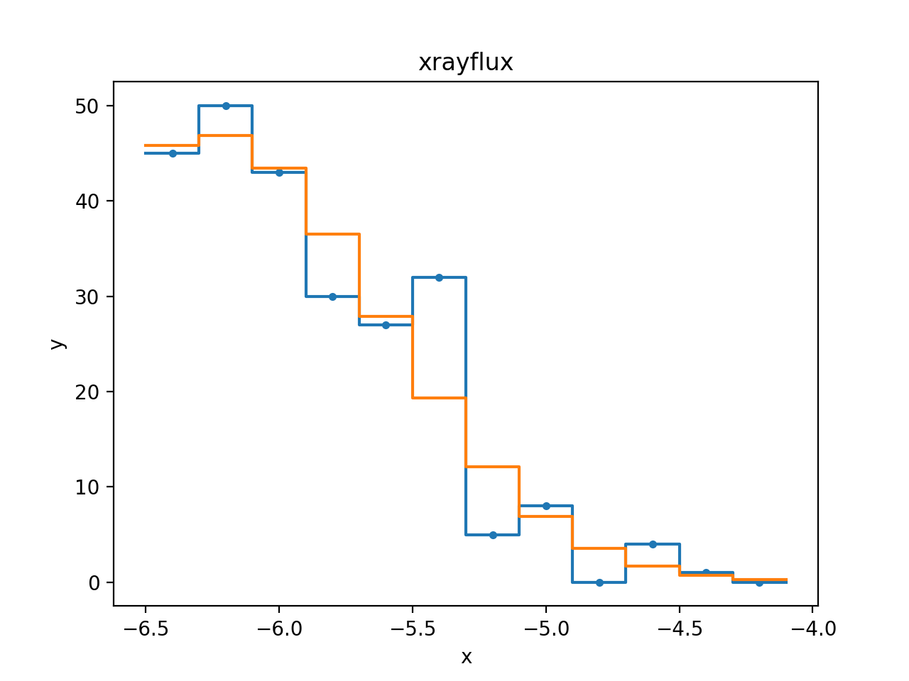
>>> from sherpa.plot import DataHistogramPlot, ModelHistogramPlot
>>> dplot = DataHistogramPlot()
>>> dplot.prepare(xfit.data)
>>> mplot = ModelHistogramPlot()
>>> mplot.prepare(xfit.data, xfit.model)
>>> dplot.plot(linestyle='solid')
>>> mplot.overplot()

Dealing with negative models
This sample dataset contains a continuum with line emission, modelled
as a delta function. The signal is such that it is easy to end up with
the amplitude of either the continuum or line going negative, which
causes problems with CStat.
>>> from sherpa.astro.io import read_pha, read_rmf
>>> from sherpa.astro.plot import DataPHAPlot
>>> pha = read_pha("P0112880201R2S005SRSPEC1003.FTZ")
>>> rmf = read_rmf("P0112880201R2S005RSPMAT1003.FTZ")
>>> pha.set_rmf(rmf)
>>> pha.set_analysis("wave")
>>> pha.notice(11.4, 11.7)
>>> pha.group_counts(1)
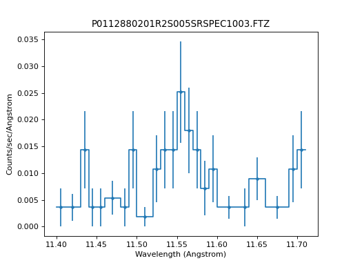
>>> dplot = DataPHAPlot()
>>> stat1 = CStat()
>>> dplot.prepare(pha, stat=stat1)
>>> dplot.plot(linestyle="-", yerrorbars=True)

As this is a PHA dataset, the source model needs to include the
instrument response, calculated here with
get_full_response():
>>> from sherpa.models.basic import Const1D, Delta1D
>>> bkg = Const1D('bkg')
>>> line = Delta1D('line')
>>> line.pos.set(11.5467, frozen=True)
>>> rsp = pha.get_full_response()
>>> source = rsp(bkg + line)
>>> method = NelderMead()
When fitting with CStat, the fit ends up
stuck with a negative amplitude for the line:
>>> bkg.c0 = 7e-4
>>> line.ampl = 5e-2
>>> fit1 = Fit(pha, source, stat=stat1, method=method)
>>> res1 = fit1.fit()
>>> print(res1.format())
Method                = neldermead
Statistic             = cstat
Initial fit statistic = 116234
Final fit statistic   = 7976.99 at function evaluation 329
Data points           = 23
Degrees of freedom    = 21
Probability [Q-value] = 0
Reduced statistic     = 379.857
Change in statistic   = 108257
   bkg.c0         0.0007
   line.ampl      -1.15
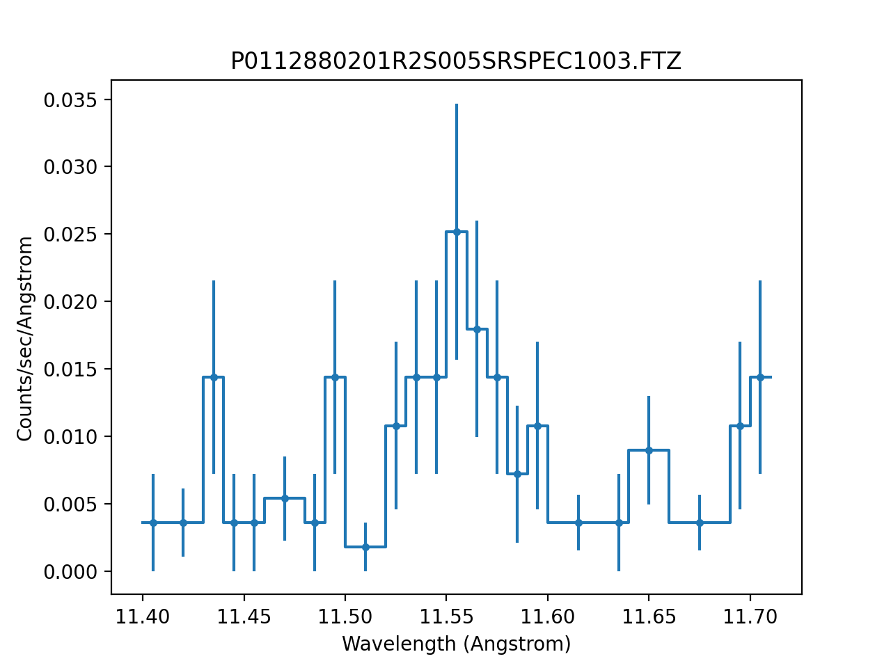
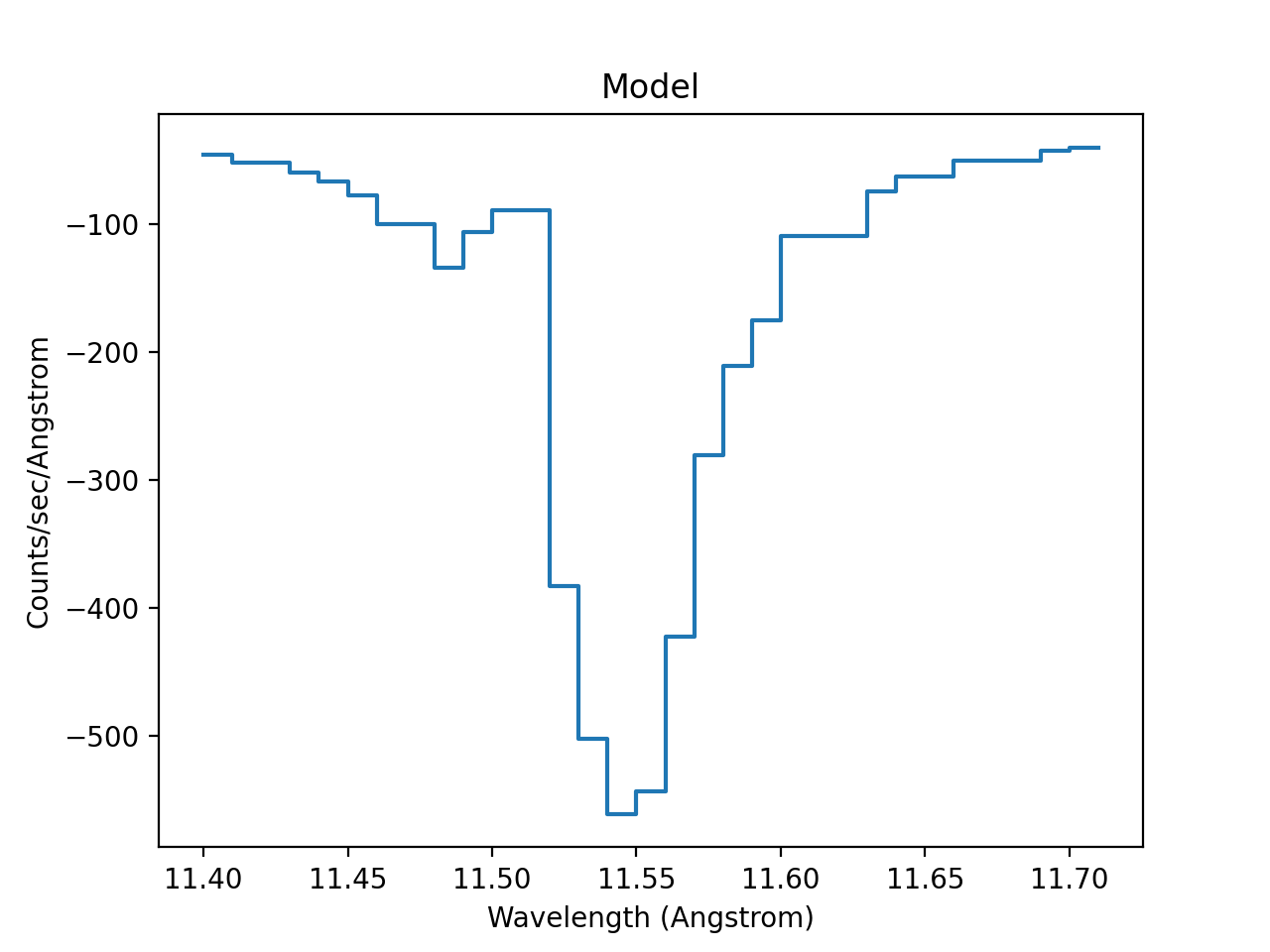
This has happened because the model has ended up predicting negative values for this set of parameters:
>>> from sherpa.astro.plot import ModelPHAHistogram
>>> mplot = ModelPHAHistogram()
>>> mplot.prepare(pha, source)
>>> mplot.plot()
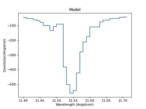
The CStat statistic replaces these negative
predicted values with a constant term, and so the optimisation gets
stuck. When using CStatNegativePenalty the
optimiser is able to move the fit back into parts of the parameter
space where the predicted model values are positive:
>>> stat2 = CStatNegativePenalty()
>>> bkg.c0 = 7e-4
>>> line.ampl = 5e-2
>>> fit2 = Fit(pha, source, stat=stat2, method=method)
>>> res2 = fit2.fit()
>>> print(res2.format())
Method                = neldermead
Statistic             = cstatnegativepenalty
Initial fit statistic = 116234
Final fit statistic   = 17.816 at function evaluation 445
Data points           = 23
Degrees of freedom    = 21
Probability [Q-value] = 0.660615
Reduced statistic     = 0.848382
Change in statistic   = 116216
   bkg.c0         7.69918e-05
   line.ampl      2.83667e-05
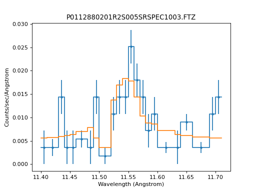
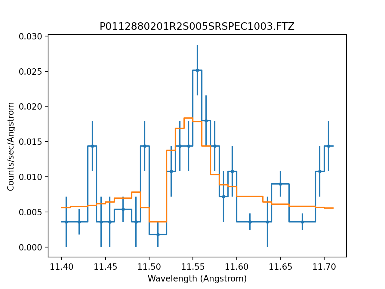
The resulting fit is a close match to the data:
>>> dplot = DataPHAPlot()
>>> dplot.prepare(pha, stat=stat2)
>>> mplot = ModelPHAHistogram()
>>> mplot.prepare(pha, source)
>>> dplot.plot(linestyle="-", yerrorbars=True)
>>> mplot.overplot()