Analyzing PHA data
As mentioned in Accessing filtered data, PHA datasets add extra features to the standard Sherpa data class. These are:
creating a PHA data set requires significantly more metadata than other data classes, which is automatically handled when reading the data from a FITS file that follows the OGIP standards, but have to be explicitly set when creating a
DataPHAobject;the
sherpa.astro.data.DataPHAclass is derived fromsherpa.data.Data1D, since the “raw” data being fit is channel number and counts, but much analysis requires an “integrated” data set;a source region can also have one or more associated background regions which provide an estimate of the background contamination in the source region and this can either be subtracted from the data or a separate model fit to it;
analysis can be done using one of three “coordinates” -
"channel","energy", or"wavelength"- that control the plot appearance and units for thenotice()andignore()calls;data can be dynamically regrouped to change the signal-to-noise during the analysis;
and model evaluation uses classes related to the ARF and RMF to convert between channels and energies.
The X-ray data (DataPHA) section of the model evaluation page shows how many of these features work, while below we focus on an overview of these changes.
The following imports have been made:
>>> import numpy as np
>>> from matplotlib import pyplot as  plt
>>> from sherpa.astro.data import DataPHA
Creating a DataPHA object
The sherpa.astro.io.read_pha() routine will read in a
PHA FITS file:
>>> from sherpa.astro.io import read_pha
>>> pha = read_pha('3c273.pi')
WARNING: systematic errors were not found in file '3c273.pi'
statistical errors were found in file '3c273.pi'
but not used; to use them, re-read with use_errors=True
read ARF file 3c273.arf
read RMF file 3c273.rmf
WARNING: systematic errors were not found in file '3c273_bg.pi'
statistical errors were found in file '3c273_bg.pi'
but not used; to use them, re-read with use_errors=True
read background file 3c273_bg.pi
>>> print(pha)
name           = 3c273.pi
channel        = Float64[1024]
counts         = Float64[1024]
staterror      = None
syserror       = None
bin_lo         = None
bin_hi         = None
grouping       = Int16[1024]
quality        = Int16[1024]
exposure       = 38564.608926889
backscal       = 2.5264364698914e-06
areascal       = 1.0
grouped        = True
subtracted     = False
units          = energy
rate           = True
plot_fac       = 0
response_ids   = [1]
background_ids = [1]
Note
The sherpa.astro.io module requires that a FITS backend
is available. The Astropy package can be used for this.
As well as reading in the data it has also automatically loaded in the background data and response information (ARF and RMF) that are set in this file’s FITS metdata:
>>> print(pha.get_background())
name           = 3c273_bg.pi
channel        = Float64[1024]
counts         = Float64[1024]
staterror      = None
syserror       = None
bin_lo         = None
bin_hi         = None
grouping       = Int16[1024]
quality        = Int16[1024]
exposure       = 38564.608926889
backscal       = 1.872535141462e-05
areascal       = 1.0
grouped        = True
subtracted     = False
units          = energy
rate           = True
plot_fac       = 0
response_ids   = [1]
background_ids = []
>>> print(pha.get_arf())
name     = 3c273.arf
energ_lo = Float64[1090]
energ_hi = Float64[1090]
specresp = Float64[1090]
bin_lo   = None
bin_hi   = None
exposure = 38564.141454905
ethresh  = 1e-10
>>> print(pha.get_rmf())
name     = 3c273.rmf
detchans = 1024
energ_lo = Float64[1090]
energ_hi = Float64[1090]
n_grp    = UInt64[1090]
f_chan   = UInt64[2002]
n_chan   = UInt64[2002]
matrix   = Float64[61834]
offset   = 1
e_min    = Float64[1024]
e_max    = Float64[1024]
ethresh  = 1e-10
A PHA object can also be created directly - all that is needed at
first are the channel and counts arrays as other metadata can be added
after the DataPHA object has been
created:
>>> chans = np.arange(1, 1025, dtype=int)
>>> counts = np.ones(1024, dtype=int)
>>> test = DataPHA('example', chans, counts)
>>> print(test)
name           = example
channel        = Int64[1024]
counts         = Int64[1024]
staterror      = None
syserror       = None
bin_lo         = None
bin_hi         = None
grouping       = None
quality        = None
exposure       = None
backscal       = None
areascal       = None
grouped        = False
subtracted     = False
units          = channel
rate           = True
plot_fac       = 0
response_ids   = []
background_ids = []
Visualizing the data
The sherpa.astro.plot module contains classes for
visualizing the data (the visualization section provides more information on how to use the
plot classes), so we
can visualize the data with:
>>> from sherpa.astro.plot import DataPHAPlot
>>> plot = DataPHAPlot()
>>> plot.histo_prefs['linestyle'] = '-'
>>> plot.prepare(pha)
>>> plot.plot()
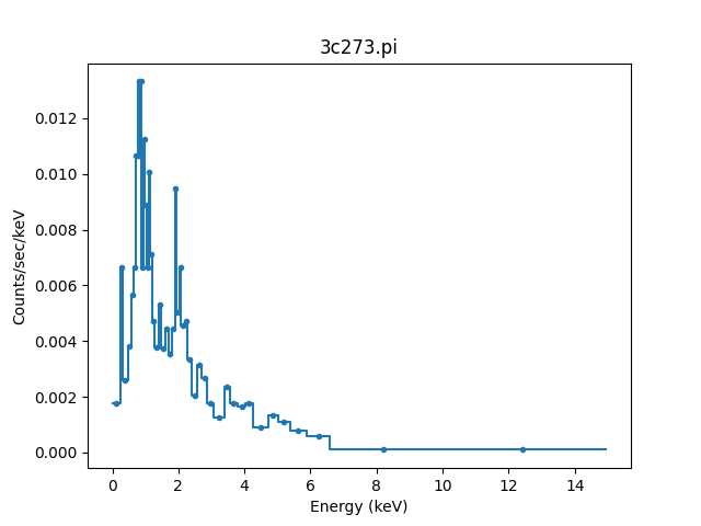
Note
The sherpa.astro.plot module requires that a plotting backend
is available. The matplotlib package can be used for this.
The default plot style has been adjusted to also include the
bin edges (by setting the matplotlib linestyle option).
Analysis units
The “native” units for analyzing PHA data is in channel space, but this is often not the most instructive, so normally the analysis is done with energy or wavelength units. If a PHA file is loaded in from disk and contains a response then it will default to energy units, otherwise it will use channel units.
For this example, the 3c273.pi file includes response information in
its header - via the RESPFILE and ANCRFILE keywords - and so
the selected units are energy, which can be found using either the
get_analysis() method or the
units attribute:
>>> pha.get_analysis()
'energy'
>>> print(pha.units)
energy
The set_analysis method or
units attribute can be
used to switch between channel, energy, and wavelength
(the latter two will raise an error if no response has been set).
Filtering
The default is for all the data to be included and, because the file contained grouping information, the data has been grouped (this is shown in the plot above, where there are only of order 50 data points shown rather than the 1024 channels this data set has):
>>> print(pha.mask)
True
>>> print(pha.grouped)
True
The “dependent axis” - so in this case, the counts - can be retrieved
with the get_dep() method, and we
can see the difference the filter flag makes:
>>> y1 = pha.get_dep()
>>> y2 = pha.get_dep(filter=True)
>>> print(y1.size)
1024
>>> print(y2.size)
46
So when filter=False (the default) then the ungrouped data is returned,
but when filter=True the grouped data is returned.
Since the analysis units for this data set are energy, we can select
a subset of the data, which means that the grouped data size is reduced,
as the points with energies below 0.5 keV or above 7 keV have been removed:
>>> pha.notice(0.5, 7)
>>> print(pha.get_dep(filter=True).size)
42
>>> plot.prepare(pha)
>>> plot.plot()
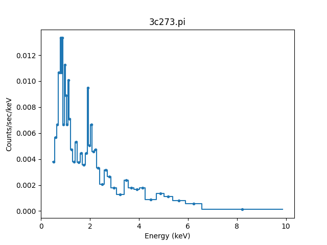
Although the requested range was 0.5 to 7.0 keV, the selected range
is wider, as shown above and with the get_filter()
method:
>>> print(pha.get_filter())
0.467200011015:9.869600296021
Note
Each channel covers a finite energy range, and so when determining what
value to display, the get_filter() call
uses the full range (this was changed in Sherpa 4.14.0, in earlier versions
the mid-point was used so the expression would appear to cover a smaller
range but would still reflect the same filter).
The reason for this change is two fold:
as mentioned, each channel has a finite energy range, so the selected energy range is unlikely to exactly match the requested range,
and thanks to grouping, the selected channel is unlikely to fall at the start (for the low limit) and end (for the high limit) values for the groups, so this further changes the selected limit range.
Consider the following highly-simplified case where there are 7 channels that have been grouped into 4 bins.
Channel |
Group |
Energy range (keV) |
|---|---|---|
1 |
1 |
0.10 - 0.11 |
2 |
0.11 - 0.14 |
|
3 |
2 |
0.14 - 0.16 |
4 |
0.16 - 0.20 |
|
5 |
3 |
0.20 - 0.22 |
6 |
0.22 - 0.24 |
|
7 |
4 |
0.24 - 0.26 |
In this case a filter to notice the range 0.15 to 0.21 keV would select channels 3 to 5 and then end up selecting groups 2 and 3, with the final channel selection being 3 to 6. A call to then ignore the range 0.18 to 0.19 keV would select channel 4 and hence group 2, so resulting in a final filter of just group 3 (channels 5 to 6).
We can switch temporarily to channel units and see differences in the
get_filter call and the plot:
>>> pha.units = 'channel'
>>> print(pha.get_filter())
33:676
>>> plot.prepare(pha)
>>> plot.plot(xlog=True, ylog=True)
>>> pha.units = 'energy'
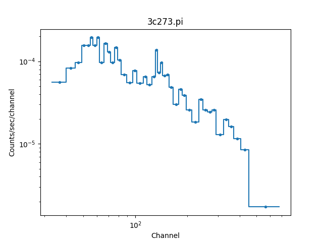
Note
The counts (dependent) axis is drawn with a logarithmic scale primarily because the values are small enough that the Y-axis label would disappear with a linear scale. The channel (independent) axis has been drawn with a log scale because the effective area of this instrument is higher at lower energies which tends to result in smaller groups at low channel values.
Filtering and limits
When using energy or wavelength units - e.g. with
set_analysis(), as
described above - the meaning of the
arguments to
notice() and
ignore() are slightly different
than when using channel units.
When using channels:
the low and high limits must be integers,
and the limits are inclusive on both ends (so
[lo, hi])
whereas for energy and wavelength analysis
the low and high limits must be >= 0,
and the limits are only inclusive on the lower value (so
[lo, hi), that is a half-open interval).
That is (for an ungrouped dataset):
>>> pha.notice()
>>> pha.units = 'channel'
>>> pha.notice(20, 200)
will select the channels 20 to 200 (inclusive), but
>>> pha.notice()
>>> pha.units = 'energy'
>>> pha.notice(0.5, 7.0)
will only select those bins which lie in the range 0.5 <= energy <
7.0 (although as just explained, the finite
width of each channel in energy or wavelength units means that the
distinction between 0.5 <= energy < 7.0 and 0.5 <= energy <=
7.0 makes no difference unless the bin edge is at 7 keV).
Note
The PHA filtering in Sherpa 4.14.0 has been updated to fix a number of corner cases which can result in filter expressions changing the first or last selected bin. This can then cause fit differences as the number of degrees of freedom and the fit parameters can change slightly.
Grouping
The dynamic grouping can be changed by setting the
grouping attribute - and
then calling the group() if
necessary - or with one of the dynamic-routines methods:
group_adapt(),
group_adapt_snr(),
group_bins(),
group_counts(),
group_snr(),
and
group_width().
For this example we will compare the same data with
different grouping schemes by loading the data in three
times. The SherpaVerbosity
class is used to temporarily hide the output of
read_pha():
>>> from sherpa.utils.logging import SherpaVerbosity
>>> with SherpaVerbosity('ERROR'):
...    pha1 = read_pha('3c273.pi')
...    pha2 = read_pha('3c273.pi')
...    pha3 = read_pha('3c273.pi')
The same energy range will be used for all three data sets:
>>> pha1.notice(0.5, 7)
>>> pha2.notice(0.5, 7)
>>> pha3.notice(0.5, 7)
The first data set is to be ungrouped, the second data set will use the on-disk grouping settings, and the third data set is grouped so that each bin contains at least 40 counts:
>>> pha1.ungroup()
>>> pha3.group_counts(40)
For display the ungrouped data is shown in a separate plot as it makes it easier to compare:
>>> plt.subplot(2, 1, 1)
>>> plot.prepare(pha1)
>>> plot.plot(clearwindow=False)
>>> plt.subplot(2, 1, 2)
>>> plot.prepare(pha2)
>>> plot.plot(xlog=True, alpha=0.7, clearwindow=False)
>>> plot.prepare(pha3)
>>> plot.overplot(alpha=0.7)
>>> plt.title('')
>>> plt.subplots_adjust(hspace=0.4)
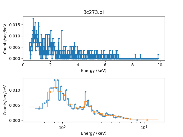
In general, as the grouped bins become larger then the difference of the filtered range to the requested range becomes larger:
>>> print(pha1.get_filter())
0.467200011015:9.869600296021
>>> print(pha2.get_filter())
0.467200011015:9.869600296021
>>> print(pha3.get_filter())
0.394199997187:14.950400352478
Manipulating data
Methods like get_dep() will apply
the necessary grouping and filters to the data. It can be useful to
convert other arrays - such as counts or energy bins - directly, which
can be done with apply_filter()
and apply_grouping(). The default
behavior for apply_filter is to sum the data values with each
group, so we can re-create the get_dep call:
>>> d1 = pha.get_dep(filter=True)
>>> d2 = pha.apply_filter(pha.counts)
>>> np.all(d1 == d2)
True
The behavior can be changed with the groupfunc argument, which
takes a limited set of functions that describe how the data within a
group is combined (the default is np.sum). For instance, the
first and last channel value of each group can be calculated with:
>>> clo = pha.apply_filter(pha.channel, groupfunc=pha._min)
>>> chi = pha.apply_filter(pha.channel, groupfunc=pha._max)
>>> clo[0:7]
[33. 40. 45. 49. 52. 55. 57.]
>>> chi[0:7]
[39. 44. 48. 51. 54. 56. 59.]
The apply_grouping() method is
similar but it does not apply any filter, so all channels are used. So
to get the group boundaries for all channels, not just the filtered
ones, we can say:
>>> alo = pha.apply_grouping(pha.channel, pha._min)
>>> ahi = pha.apply_grouping(pha.channel, pha._max)
>>> alo[0:7]
[ 1. 18. 22. 33. 40. 45. 49.]
>>> ahi[0:7]
[17. 21. 32. 39. 44. 48. 51.]
Background
A PHA data set may have one or more associated background
data sets. For this example there is one, and the
get_background() method
will return a DataPHA object
representing the background region.
>>> print(pha.background_ids)
[1]
>>> bkg = pha.get_background()
>>> print(bkg)
name           = 3c273_bg.pi
channel        = Float64[1024]
counts         = Float64[1024]
staterror      = None
syserror       = None
bin_lo         = None
bin_hi         = None
grouping       = Int16[1024]
quality        = Int16[1024]
exposure       = 38564.608926889
backscal       = 1.872535141462e-05
areascal       = 1.0
grouped        = True
subtracted     = False
units          = energy
rate           = True
plot_fac       = 0
response_ids   = [1]
background_ids = []
Note
In this example the background data has the same exposure time as the source, which is often the case (the source and background spectra are extracted from the same event file), but this does not need to hold.
Often all that is done is to subtract the background from the source data,
which is achieved with the subtract()
method, but you can instead fit a model to just the background data, and
have this then included in the source region (with appropriate scaling
to account for differences in the source and background apertures). Filtering
and grouping changes to a source region are automatically propogated to
the associated background regions, but they can be applied to the background
data set directly if needed.
For example, the un-subtracted group counts are:
>>> pha.get_dep(filter=True)
[15. 16. 15. 18. 18. 15. 18. 15. 15. 19. 15. 15. 17. 16. 16. 17. 15. 19.
 15. 16. 15. 16. 17. 15. 18. 16. 15. 15. 16. 15. 15. 15. 16. 16. 15. 15.
 16. 16. 15. 16. 15. 15.]
and after background subtractuion the values are:
>>> pha.subtract()
>>> pha.get_dep(filter=True)
[14.86507936 15.86507936 15.         18.         18.         14.86507936
 17.86507936 15.         14.59523807 18.86507936 14.86507936 14.86507936
 17.         16.         15.73015871 16.73015871 15.         18.59523807
 14.86507936 15.59523807 14.86507936 16.         16.59523807 15.
 17.59523807 16.         15.         14.46031742 16.         14.59523807
 14.59523807 14.46031742 15.86507936 15.59523807 14.32539678 14.32539678
 15.32539678 15.19047614 14.32539678 15.19047614 14.05555549 12.43650777]