Writing your own model
A model class can be created to fit any function, or interface with external code.
A one-dimensional model
An example is the AstroPy trapezoidal model, which has four parameters: the amplitude of the central region, the center and width of this region, and the slope. The following model class, which was not written for efficiancy or robustness, implements this interface:
import numpy as np

from sherpa.models import model

__all__ = ('Trap1D', )


def _trap1d(pars, x):
    """Evaluate the Trapezoid.

    Parameters
    ----------
    pars: sequence of 4 numbers
        The order is amplitude, center, width, and slope.
        These numbers are assumed to be valid (e.g. width
        is 0 or greater).
    x: sequence of numbers
        The grid on which to evaluate the model. It is expected
        to be a floating-point type.

    Returns
    -------
    y: sequence of numbers
        The model evaluated on the input grid.

    Notes
    -----
    This is based on the interface described at
    https://docs.astropy.org/en/stable/api/astropy.modeling.functional_models.Trapezoid1D.html
    but implemented without looking at the code, so any errors
    are not due to AstroPy.
    """

    (amplitude, center, width, slope) = pars

    # There are five segments:
    #    xlo = center - width/2
    #    xhi = center + width/2
    #    x0  = xlo - amplitude/slope
    #    x1  = xhi + amplitude/slope
    #
    #    flat   xlo <= x < xhi
    #    slope  x0 <= x < xlo
    #           xhi <= x < x1
    #    zero   x < x0
    #           x >= x1
    #
    hwidth = width / 2.0
    dx = amplitude / slope
    xlo = center - hwidth
    xhi = center + hwidth
    x0 = xlo - dx
    x1 = xhi + dx

    out = np.zeros(x.size)
    out[(x >= xlo) & (x < xhi)] = amplitude

    idx = np.where((x >= x0) & (x < xlo))
    out[idx] = slope * x[idx] - slope * x0

    idx = np.where((x >= xhi) & (x < x1))
    out[idx] = - slope * x[idx] + slope * x1

    return out


class Trap1D(model.RegriddableModel1D):
    """A one-dimensional trapezoid.

    The model parameters are:

    ampl
        The amplitude of the central (flat) segment (zero or greater).
    center
        The center of the central segment.
    width
        The width of the central segment (zero or greater).
    slope
        The gradient of the slopes (zero or greater).

    """

    def __init__(self, name='trap1d'):
        self.ampl = model.Parameter(name, 'ampl', 1, min=0, hard_min=0)
        self.center = model.Parameter(name, 'center', 1)
        self.width = model.Parameter(name, 'width', 1, min=0, hard_min=0)
        self.slope = model.Parameter(name, 'slope', 1, min=0, hard_min=0)

        model.RegriddableModel1D.__init__(self, name,
                                          (self.ampl, self.center, self.width,
                                           self.slope))

    def calc(self, pars, x, *args, **kwargs):
        """Evaluate the model"""

        # If given an integrated data set, use the center of the bin
        if len(args) == 1:
            x = (x + args[0]) / 2

        return _trap1d(pars, x)
This can be used in the same manner as the
Gauss1D model
in the quick guide to Sherpa.
First, create the data to fit:
>>> import numpy as np
>>> import matplotlib.pyplot as plt
>>> np.random.seed(0)
>>> x = np.linspace(-5., 5., 200)
>>> ampl_true = 3
>>> pos_true = 1.3
>>> sigma_true = 0.8
>>> err_true = 0.2
>>> y = ampl_true * np.exp(-0.5 * (x - pos_true)**2 / sigma_true**2)
>>> y += np.random.normal(0., err_true, x.shape)
Now create a Sherpa data object:
>>> from sherpa.data import Data1D
>>> d = Data1D('example', x, y)
Set up the user model:
>>> from trap import Trap1D
>>> t = Trap1D()
>>> print(t)
trap1d
   Param        Type          Value          Min          Max      Units
   -----        ----          -----          ---          ---      -----
   trap1d.ampl  thawed            1            0  3.40282e+38
   trap1d.center thawed            1 -3.40282e+38  3.40282e+38
   trap1d.width thawed            1            0  3.40282e+38
   trap1d.slope thawed            1            0  3.40282e+38
Finally, perform the fit:
>>> from sherpa.fit import Fit
>>> from sherpa.stats import LeastSq
>>> from sherpa.optmethods import LevMar
>>> tfit = Fit(d, t, stat=LeastSq(), method=LevMar())
>>> tres = tfit.fit()
>>> if not tres.succeeded: print(tres.message)
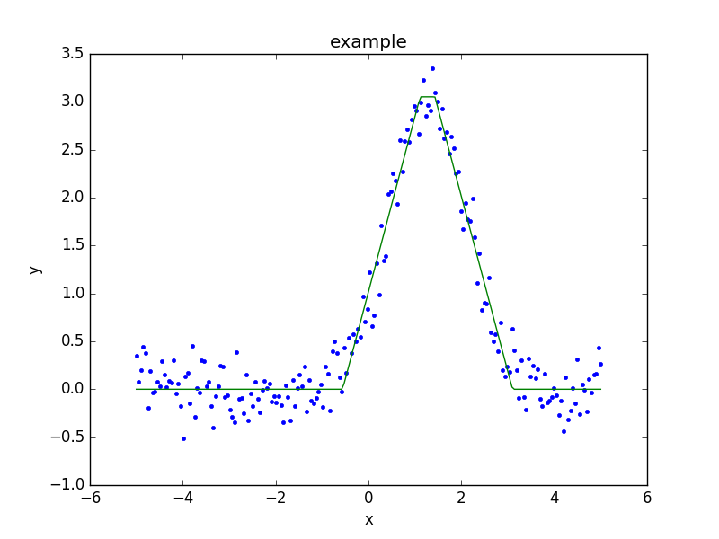
Rather than use a ModelPlot object,
the overplot argument can be set to allow multiple values
in the same plot:
>>> from sherpa import plot
>>> dplot = plot.DataPlot()
>>> dplot.prepare(d)
>>> dplot.plot()
>>> mplot = plot.ModelPlot()
>>> mplot.prepare(d, t)
>>> mplot.plot(overplot=True)
A two-dimensional model
The two-dimensional case is similar to the one-dimensional case,
with the major difference being the number of independent axes to
deal with. In the following example the model is assumed to only be
applied to non-integrated data sets, as it simplifies the implementation
of the calc method.
It also shows one way of embedding models from a different system, in this case the two-dimemensional polynomial model from the AstroPy package.
from sherpa.models import model
from astropy.modeling.polynomial import Polynomial2D

__all__ = ('WrapPoly2D', )


class WrapPoly2D(model.RegriddableModel2D):
    """A two-dimensional polynomial from AstroPy, restricted to degree=2.

    The model parameters (with the same meaning as the underlying
    AstroPy model) are:

    c0_0
    c1_0
    c2_0
    c0_1
    c0_2
    c1_1

    """

    def __init__(self, name='wrappoly2d'):
        self._actual = Polynomial2D(degree=2)
        self.c0_0 = model.Parameter(name, 'c0_0', 0)
        self.c1_0 = model.Parameter(name, 'c1_0', 0)
        self.c2_0 = model.Parameter(name, 'c2_0', 0)
        self.c0_1 = model.Parameter(name, 'c0_1', 0)
        self.c0_2 = model.Parameter(name, 'c0_2', 0)
        self.c1_1 = model.Parameter(name, 'c1_1', 0)

        model.RegriddableModel2D.__init__(self, name,
                                          (self.c0_0, self.c1_0, self.c2_0,
                                           self.c0_1, self.c0_2, self.c1_1))

    def calc(self, pars, x0, x1, *args, **kwargs):
        """Evaluate the model"""

        # This does not support 2D integrated data sets
        mdl = self._actual
        for n in ['c0_0', 'c1_0', 'c2_0', 'c0_1', 'c0_2', 'c1_1']:
            pval = getattr(self, n).val
            getattr(mdl, n).value = pval

        return mdl(x0, x1)
Repeating the 2D fit by first setting up the data to fit:
>>> np.random.seed(0)
>>> y2, x2 = np.mgrid[:128, :128]
>>> z = 2. * x2 ** 2 - 0.5 * y2 ** 2 + 1.5 * x2 * y2 - 1.
>>> z += np.random.normal(0., 0.1, z.shape) * 50000.
Put this data into a Sherpa data object:
>>> from sherpa.data import Data2D
>>> x0axis = x2.ravel()
>>> x1axis = y2.ravel()
>>> d2 = Data2D('img', x0axis, x1axis, z.ravel(), shape=(128,128))
Create an instance of the user model:
>>> from poly import WrapPoly2D
>>> wp2 = WrapPoly2D('wp2')
>>> wp2.c1_0.frozen = True
>>> wp2.c0_1.frozen = True
Finally, perform the fit:
>>> f2 = Fit(d2, wp2, stat=LeastSq(), method=LevMar())
>>> res2 = f2.fit()
>>> if not res2.succeeded: print(res2.message)
>>> print(res2)
datasets       = None
itermethodname = none
methodname     = levmar
statname       = leastsq
succeeded      = True
parnames       = ('wp2.c0_0', 'wp2.c2_0', 'wp2.c0_2', 'wp2.c1_1')
parvals        = (-80.289475553599914, 1.9894112623565667, -0.4817452191363118, 1.5022711710873158)
statval        = 400658883390.6685
istatval       = 6571934382318.328
dstatval       = 6.17127549893e+12
numpoints      = 16384
dof            = 16380
qval           = None
rstat          = None
message        = successful termination
nfev           = 80
>>> print(wp2)
wp2
   Param        Type          Value          Min          Max      Units
   -----        ----          -----          ---          ---      -----
   wp2.c0_0     thawed     -80.2895 -3.40282e+38  3.40282e+38
   wp2.c1_0     frozen            0 -3.40282e+38  3.40282e+38
   wp2.c2_0     thawed      1.98941 -3.40282e+38  3.40282e+38
   wp2.c0_1     frozen            0 -3.40282e+38  3.40282e+38
   wp2.c0_2     thawed    -0.481745 -3.40282e+38  3.40282e+38
   wp2.c1_1     thawed      1.50227 -3.40282e+38  3.40282e+38