Markov Chain Monte Carlo and Poisson data¶

Sherpa provides a Markov Chain Monte Carlo (MCMC) method designed for Poisson-distributed data. It was originally developed as the Bayesian Low-Count X-ray Spectral (BLoCXS) package, but has since been incorporated into Sherpa. It is developed from the work presented in Analysis of Energy Spectra with Low Photon Counts via Bayesian Posterior Simulation by van Dyk et al. (2001).

Markov chain Monte Carlo (MCMC) selects random samples from the posterior probability distribution of the model parameters starting from the best fit (maximum likelihood) given by the standard optimization methods in Sherpa (i.e. result of the fit()). get_draws() runs MCMC chains for a specific dataset, the selected sampler, the priors, and the specified number of iterations. It returns an array of statistic values, an array of acceptance Booleans, and an array of sampled parameter values (i.e. draws) from the posterior distribution.

The multivariate t-distribution is the default sampling distribution in get_draws(). This distribution is defined by the multivariate normal (for the model parameter values and the covariance matrix), and chi2 distribution for a given degrees of freedom. The algorithm provides a choice of MCMC samplers with different jumping rules for a selection of the proposed parameters: Metropolis (symmetric) and Metropolis-Hastings (asymmetric).

Note that the multivariate normal distribution which requires the parameter values and the corresponding covariance matrix. covar() should be run beforehand.

Additional scale parameter allows to adjust the scale size of the multivariate normal in the definition of the t-distribution. This could improve the efficiency of the sampler and can be used to obtain the required acceptance rates.

Example¶

Note

This example probably needs to be simplified to reduce the run time

Simulate the data¶

Create a simulated data set:

>>> np.random.seed(2)
>>> x0low, x0high = 3000, 4000
>>> x1low, x1high = 4000, 4800
>>> dx = 15
>>> x1, x0 = np.mgrid[x1low:x1high:dx, x0low:x0high:dx]

Convert to 1D arrays:

>>> shape = x0.shape
>>> x0, x1 = x0.flatten(), x1.flatten()

Create the model used to simulate the data:

>>> from sherpa.astro.models import Beta2D
>>> truth = Beta2D()
>>> truth.xpos, truth.ypos = 3512, 4418
>>> truth.r0, truth.alpha = 120, 2.1
>>> truth.ampl = 12

Evaluate the model to calculate the expected values:

>>> mexp = truth(x0, x1).reshape(shape)

Create the simulated data by adding in Poisson-distributed noise:

>>> msim = np.random.poisson(mexp)

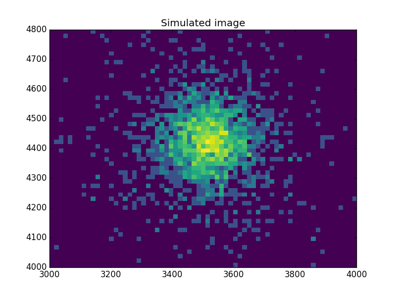
What does the data look like?¶

Use an arcsinh transform to view the data, based on the work of Lupton, Gunn & Szalay (1999).

>>> plt.imshow(np.arcsinh(msim), origin='lower', cmap='viridis',
...            extent=(x0low, x0high, x1low, x1high),
...            interpolation='nearest', aspect='auto')
>>> plt.title('Simulated image')

Find the starting point for the MCMC¶

Set up a model and use the standard Sherpa approach to find a good starting place for the MCMC analysis:

>>> from sherpa import data, stats, optmethods, fit
>>> d = data.Data2D('sim', x0, x1, msim.flatten(), shape=shape)
>>> mdl = Beta2D()
>>> mdl.xpos, mdl.ypos = 3500, 4400

Use a Likelihood statistic and Nelder-Mead algorithm:

>>> f = fit.Fit(d, mdl, stats.Cash(), optmethods.NelderMead())
>>> res = f.fit()
>>> print(res.format())
Method                = neldermead
Statistic             = cash
Initial fit statistic = 20048.5
Final fit statistic   = 607.229 at function evaluation 777
Data points           = 3618
Degrees of freedom    = 3613
Change in statistic   = 19441.3
   beta2d.r0      121.945
   beta2d.xpos    3511.99
   beta2d.ypos    4419.72
   beta2d.ampl    12.0598
   beta2d.alpha   2.13319

Now calculate the covariance matrix (the default error estimate):

>>> f.estmethod
<Covariance error-estimation method instance 'covariance'>
>>> eres = f.est_errors()
>>> print(eres.format())
Confidence Method     = covariance
Iterative Fit Method  = None
Fitting Method        = neldermead
Statistic             = cash
covariance 1-sigma (68.2689%) bounds:
   Param            Best-Fit  Lower Bound  Upper Bound
   -----            --------  -----------  -----------
   beta2d.r0         121.945     -7.12579      7.12579
   beta2d.xpos       3511.99     -2.09145      2.09145
   beta2d.ypos       4419.72     -2.10775      2.10775
   beta2d.ampl       12.0598    -0.610294     0.610294
   beta2d.alpha      2.13319    -0.101558     0.101558

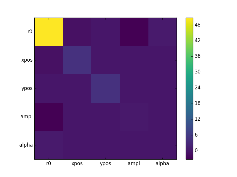
The covariance matrix is stored in the extra_output attribute:

>>> cmatrix = eres.extra_output
>>> pnames = [p.split('.')[1] for p in eres.parnames]
>>> plt.imshow(cmatrix, interpolation='nearest', cmap='viridis')
>>> plt.xticks(np.arange(5), pnames)
>>> plt.yticks(np.arange(5), pnames)
>>> plt.colorbar()

Run the chain¶

Finally, run a chain (use a small number to keep the run time low for this example):

>>> from sherpa.sim import MCMC
>>> mcmc = MCMC()
>>> mcmc.get_sampler_name()
>>> draws = mcmc.get_draws(f, cmatrix, niter=1000)
>>> svals, accept, pvals = draws

>>> pvals.shape
(5, 1001)
>>> accept.sum() * 1.0 / 1000
0.48499999999999999

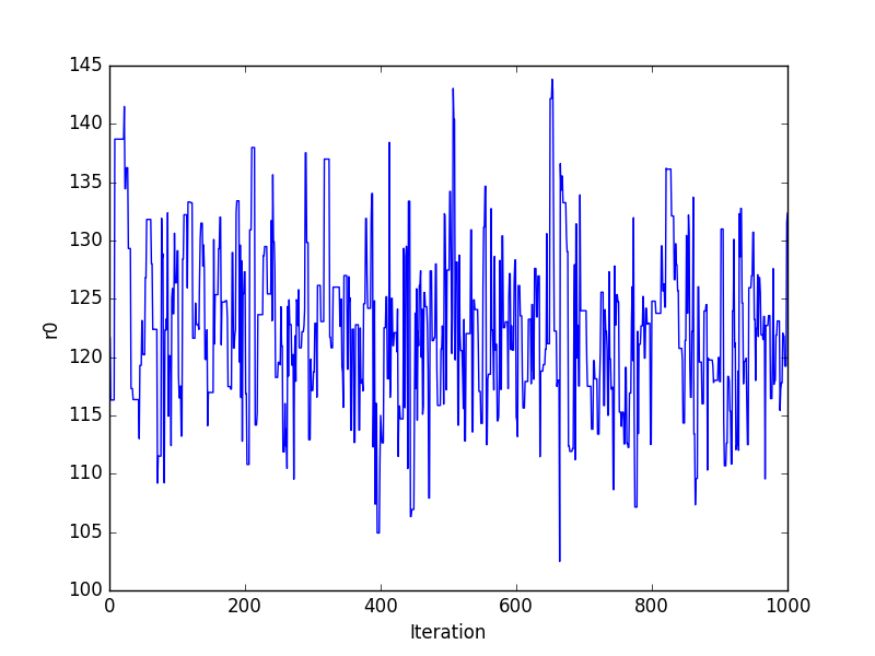
Trace plots¶

>>> plt.plot(pvals[0, :])
>>> plt.xlabel('Iteration')
>>> plt.ylabel('r0')

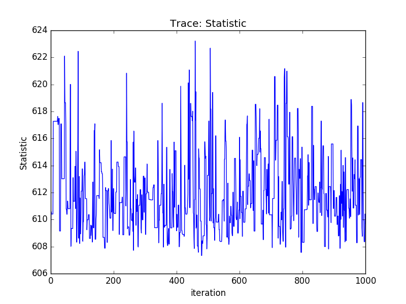
Or using the sherpa.plot module:

>>> from sherpa import plot
>>> tplot = plot.TracePlot()
>>> tplot.prepare(svals, name='Statistic')
>>> tplot.plot()

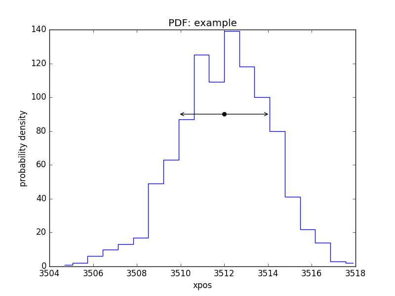
PDF of a parameter¶

>>> pdf = plot.PDFPlot()
>>> pdf.prepare(pvals[1, :], 20, False, 'xpos', name='example')
>>> pdf.plot()

Add in the covariance estimate:

>>> xlo, xhi = eres.parmins[1] + eres.parvals[1], eres.parmaxes[1] + eres.parvals[1]

>>> plt.annotate('', (xlo, 90), (xhi, 90), arrowprops={'arrowstyle': '<->'})
>>> plt.plot([eres.parvals[1]], [90], 'ok')

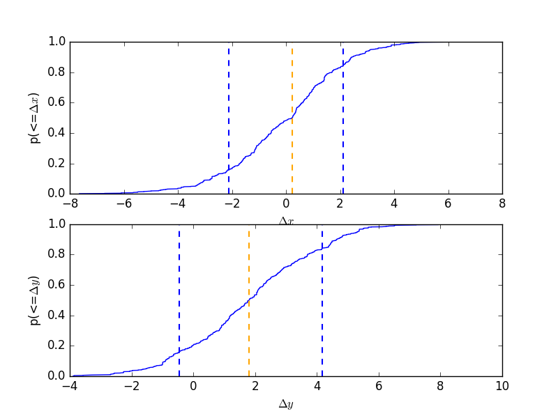
CDF for a parameter¶

Normalise by the actual answer to make it easier to see how well the results match reality:

>>> cdf = plot.CDFPlot()
>>> plt.subplot(2, 1, 1)
>>> cdf.prepare(pvals[1, :] - truth.xpos.val, r'$\Delta x$')
>>> cdf.plot(clearwindow=False)
>>> plt.title('')
>>> plt.subplot(2, 1, 2)
>>> cdf.prepare(pvals[2, :] - truth.ypos.val, r'$\Delta y$')
>>> cdf.plot(clearwindow=False)
>>> plt.title('')

Scatter plot¶

>>> plt.scatter(pvals[0, :] - truth.r0.val,
...             pvals[4, :] - truth.alpha.val, alpha=0.3)
>>> plt.xlabel(r'$\Delta r_0$', size=18)
>>> plt.ylabel(r'$\Delta \alpha$', size=18)

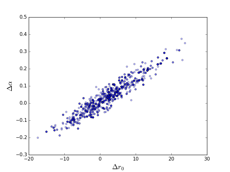
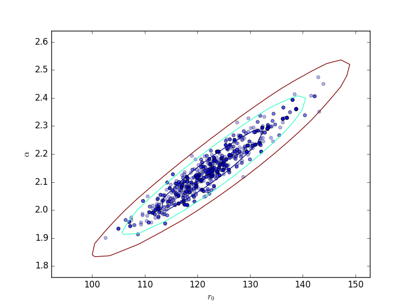
This can be compared to the RegionProjection calculation:

>>> plt.scatter(pvals[0, :], pvals[4, :], alpha=0.3)

>>> from sherpa.plot import RegionProjection
>>> rproj = RegionProjection()
>>> rproj.prepare(min=[95, 1.8], max=[150, 2.6], nloop=[21, 21])
>>> rproj.calc(f, mdl.r0, mdl.alpha)
>>> rproj.contour(overplot=True)
>>> plt.xlabel(r'$r_0$'); plt.ylabel(r'$\alpha$')

../_images/mcmc_scatter_r0_alpha_compare.png